TimeMixer: Exploring the Latest Model in Time Series Forecasting
Jul 23, 2024
The field of time series forecasting keeps evolving at a rapid pace, with many models being proposed and claiming state-of-the-art performance.
Deep learning models are now common methods for time series forecasting, especially on large datasets with many features.
Although numerous models have been proposed in recent years, such as the iTransformer, SOFTS, and TimesNet, their performance often falls short in other benchmarks against models like NHITS, PatchTST and TSMixer.
In May 2024, a new model was proposed: TimeMixer. According to the original paper TimeMixer: Decomposable Multiscale Mixing for Time Series Forecasting, this model uses mixing of features along with series decomposition in an MLP-based architecture to produce forecasts.
In this article, we first explore the inner workings of TimeMixer before running our own little benchmark in both short and long horizon forecasting tasks.
As always, make sure to read the original research article for more details.
Learn the latest time series forecasting techniques with my free time series cheat sheet in Python! Get the implementation of statistical and deep learning techniques, all in Python and TensorFlow!
Let’s get started!
Discover TimeMixer
The motivation behind TimeMixer comes from the realization that time series data hold different information at different scales.
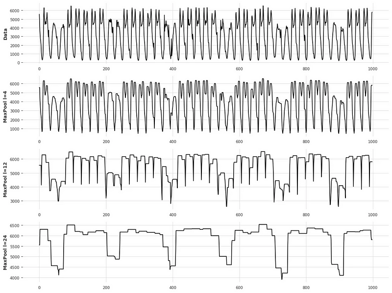
In the figure above, we can see that depending on the scale at which we sample the data, different patterns arise.
Of course, at a small sampling scale (top of the figure), we have fine variations, while at a large sampling scale (as shown in the bottom portion of the figure), we see more coarse changes to the series over a longer period of time.
Thus, TimeMixer looks to disentangle the microscopic and macroscopic information and apply feature mixing, which is an idea that was fully explored in TSMixer.
Architecture of TimeMixer
Below, we can see the general architecture of TimeMixer.
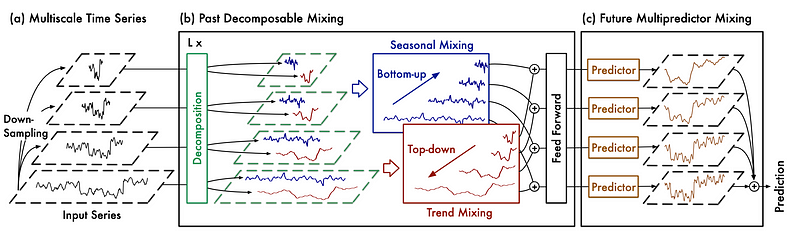
In the figure above, we see that the input series is first downsampled using average pooling. That way, we can the decouple the fine from the coarse variations in the series.
The decoupled series is then sent to the Past-Decomposable-Mixing block, or PDM block, where information at different scales is learned by the model. Notice also a further decomposition, where trend and seasonality are treated separately.
Finally, the model is sent to the Future-Multipredictor-Mixing block, or FMM block. This ensembles the prediction at each scale to get the final forecast.
Of course, there is much more information to learn about each step, so let’s cover them in more detail.
Past decomposable mixing (PDM)
The first step of average pooling the series at different scales is straightforward enough to move directly to the Past-Decomposable-Mixing block immediately.
Here, the series is further decomposed into its trend and seasonal components. Note that the seasonal component carries short-term and cyclical changes, while the trend component carries slow changes over longer periods of time.
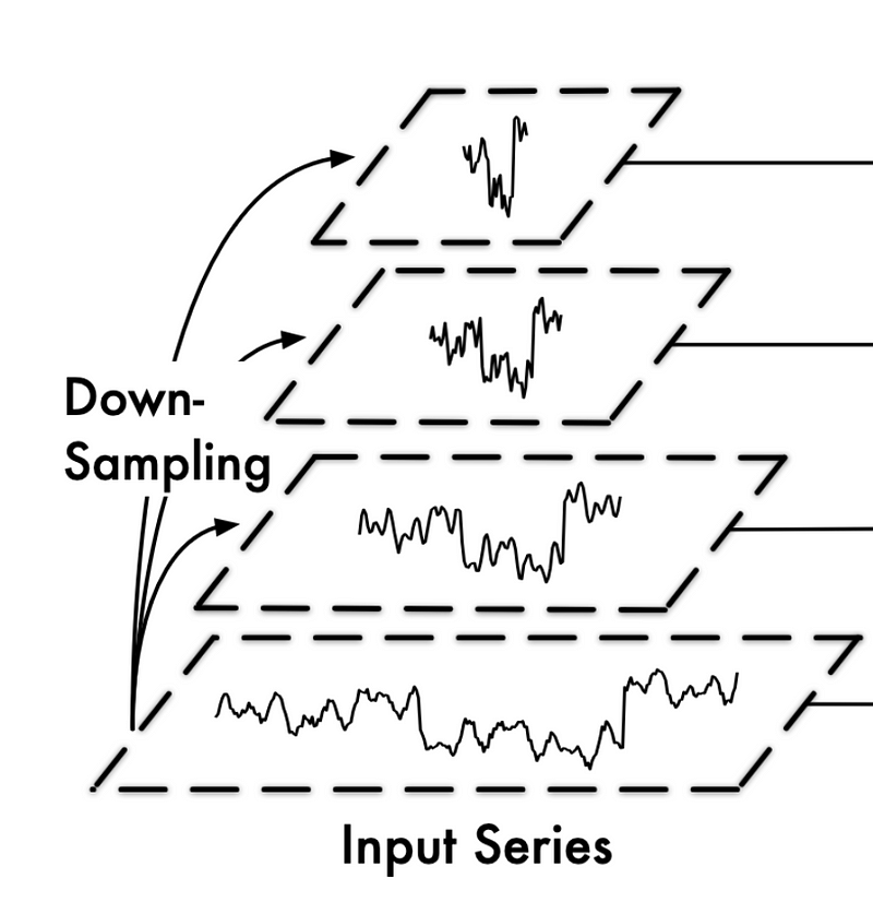
From the figure above, we can see that the top series is downsampled, but it still exhibits trend and seasonal properties. Therefore, it is beneficial to separate both components as they carry different information.
To carry out this decomposition, the researchers reuse the logic from Autoformer, which basically uses average pooling to smooth out cyclical variations, thus highlighting the trend.
This is then combined with a Fourier transform, which transforms the input series into a function of frequencies and amplitude.
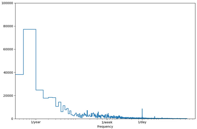
In the image above, we can see that the Fourier transform results in a function of amplitude and frequency. Frequencies at which the amplitude are the largest are then the most important, thus indicating strong seasonal effects.
Seasonal mixing
Once the trend and seasonality components are separated, they both undergo mixing.
In the case of seasonal mixing, we realize that larger seasonal periods can be seen as aggregation of smaller seasonal periods.
For example, a weekly seasonality can appear due to the daily seasonality observed in the last seven days.
Thus, TimeMixer employs a bottom-up approach to seasonal mixing.
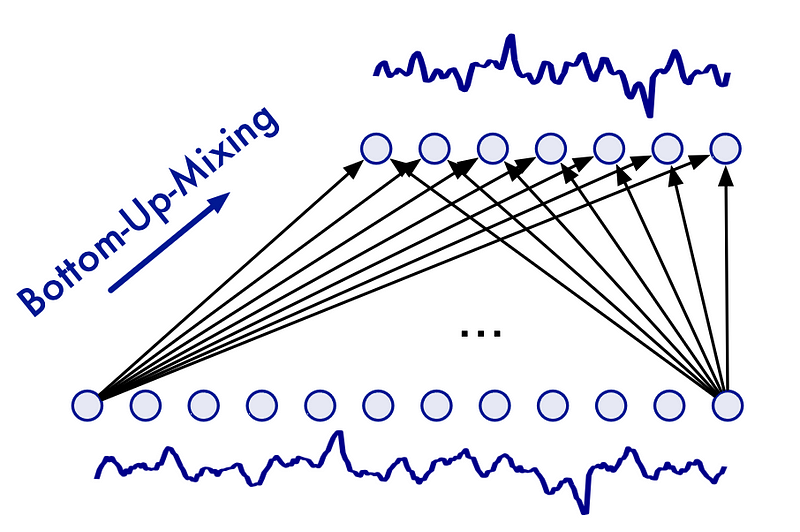
In the figure above, we can see that in seasonal mixing, we incorporate information from the fine-scale series up to the downsampled series.
Trend mixing
On the other hand, for trend mixing, TimeMixer uses a top-down approach, as shown below.
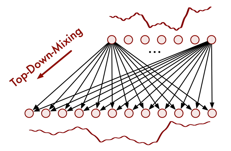
A top-down approach is used for the trend component, because noise from a fine-scale series can be introduced when trying to capture the macroscopic trend of the downsampled series.
Therefore, macro trends are used to further inform micro trends in this case.
This is how TimeMixer achieves mixing on different scales for both the trend and seasonality components.
Once this step is done, the data flows to the Future-Multipredictor-Mixing block
Future multipredictor mixing (FMM)
Here, the future-multipredictor-mixing block receives information at different scales. Therefore, it is responsible to aggregate this information to output the final prediction.
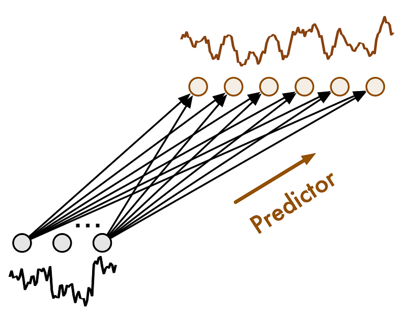
In the figure above, we can see what the FMM block looks like. Basically, because each predictor runs on a different scale, they are not all used at the same time.
For example, a predictor for on a finer scale will influence the prediction at many steps. On the other hand, a predictor on a coarse will influence the prediction at fewer time steps, since it treats downsampled data.
Now that we have a deep understanding of TimeMixer and how it works, let’s apply it in our own little benchmark using Python.
Forecasting with TimeMixer
Let’s now work with TimeMixer and evaluate in both short and long horizon forecasting tasks.
For the short horizon benchmark, we use the M3 dataset, released under the Creative Commons license. This compiles yearly, quarterly and monthly data from different domains like demography, finance, and others.
For the long horizon benchmark, we use the Electricity Transformer dataset (ETT) released under the Creative Commons License. This tracks the oil temperature of an electricity transformer from two regions in a province of China. For both regions, we have a dataset sampled at each hour and every 15 minutes, for a total of four datasets. In our case, we only use the two datasets sampled at every 15 minutes.
Again, I extended the neuralforecast library with an adapted implementation of the TimeMixer model from their official repository. That way, we have a streamlined experience for using and testing different forecasting models.
Note that at the time of writing this article, TimeMixer is not in a stable release of neuralforecast just yet.
To reproduce the results, you may need to clone the repository and work in this branch.
If the branch is merged, then you can run:
pip install git+https://github.com/Nixtla/neuralforecast.git
As always, the code for this experiment is available on GitHub.
Let’s get started!
Forecasting on a short horizon
First, let’s import the required packages. They will be used for both benchmarks. Notice that we use the datasetsforecast library to load the datasets in the format expected by neuralforecast.
import time
import pandas as pd
import numpy as np
import matplotlib.pyplot as plt

from datasetsforecast.m3 import M3
from datasetsforecast.long_horizon import LongHorizon

from neuralforecast.core import NeuralForecast
from neuralforecast.losses.pytorch import MAE, MSE
from neuralforecast.models import TimeMixer, PatchTST, iTransformer, NHITS, NBEATS

from utilsforecast.losses import mae, mse, smape
from utilsforecast.evaluation import evaluate
Then, let’s define a function that load the dataset and with the appropriate frequency and horizon.
def get_dataset(name):
    if name == 'M3-yearly':
        Y_df, *_ = M3.load("./data", "Yearly")
        horizon = 6
        freq = 'Y'
    elif name == 'M3-quarterly':
        Y_df, *_ = M3.load("./data", "Quarterly")
        horizon = 8
        freq = 'Q'
    elif name == 'M3-monthly':
        Y_df, *_ = M3.load("./data", "Monthly")
        horizon = 18
        freq = 'M'

    return Y_df, horizon, freq
Now, we can initialize our models and run the benchmark.
Here, we compare TimeMixer to NHITS and NBEATS, which are notoriously fast and accurate models in this type of task.
To run this experiment, we first initialize an empty list to store our results and start a for loop over each dataset. Once the dataset is loaded, we split it into a training and a test set.
results = []

DATASETS = ['M3-yearly', 'M3-quarterly', 'M3-monthly']

for dataset in DATASETS:

    Y_df, horizon, freq = get_dataset(dataset)

    test_df = Y_df.groupby('unique_id').tail(horizon)
    train_df = Y_df.drop(test_df.index).reset_index(drop=True)
Inside that same for loop, we initialize our models. Here, we keep the default parameters for all models. The updated code then becomes:
results = []

DATASETS = ['M3-yearly', 'M3-quarterly', 'M3-monthly']

for dataset in DATASETS:

    Y_df, horizon, freq = get_dataset(dataset)

    test_df = Y_df.groupby('unique_id').tail(horizon)
    train_df = Y_df.drop(test_df.index).reset_index(drop=True)

    timemixer_model = TimeMixer(input_size=2*horizon,
                                h=horizon,
                                n_series=1,
                                scaler_type='identity',
                                early_stop_patience_steps=3)
    nbeats_model = NBEATS(input_size=2*horizon,
                          h=horizon,
                          scaler_type='identity',
                          max_steps=1000,
                          early_stop_patience_steps=3)
    nhits_model = NHITS(input_size=2*horizon,
                        h=horizon,
                        scaler_type='identity',
                        max_steps=1000,
                        early_stop_patience_steps=3)
Notice that we train for a maximum of 1000 steps, but stop training if the loss does not improve over three training steps.
Once the models are initialized, we can fit them and make predictions. Here, we also track the time it takes to complete the training process.
The update code block is shown below.
results = []

DATASETS = ['M3-yearly', 'M3-quarterly', 'M3-monthly']

for dataset in DATASETS:

    Y_df, horizon, freq = get_dataset(dataset)

    test_df = Y_df.groupby('unique_id').tail(horizon)
    train_df = Y_df.drop(test_df.index).reset_index(drop=True)

    timemixer_model = TimeMixer(input_size=2*horizon,
                                h=horizon,
                                n_series=1,
                                scaler_type='identity',
                                early_stop_patience_steps=3)
    nbeats_model = NBEATS(input_size=2*horizon,
                          h=horizon,
                          scaler_type='identity',
                          max_steps=1000,
                          early_stop_patience_steps=3)
    nhits_model = NHITS(input_size=2*horizon,
                        h=horizon,
                        scaler_type='identity',
                        max_steps=1000,
                        early_stop_patience_steps=3)

    MODELS = [timemixer_model, nbeats_model, nhits_model]
    MODEL_NAMES = ['TimeMixer', 'NBEATS', 'NHITS']

    for i, model in enumerate(MODELS):
        nf = NeuralForecast(models=[model], freq=freq)

        start = time.time()

        nf.fit(train_df, val_size=horizon)
        preds = nf.predict()

        end = time.time()
        elapsed_time = round(end - start,0)

        preds = preds.reset_index()
        test_df = pd.merge(test_df, preds, 'left', ['ds', 'unique_id'])
All that is left to do is the evaluation of the models. Here, we use the mean absolute error (MAE) and symmetric mean absolute percentage error (sMAPE), using the utilsforecast library.
The full code block thus becomes:
results = []

DATASETS = ['M3-yearly', 'M3-quarterly', 'M3-monthly']

for dataset in DATASETS:

    Y_df, horizon, freq = get_dataset(dataset)

    test_df = Y_df.groupby('unique_id').tail(horizon)
    train_df = Y_df.drop(test_df.index).reset_index(drop=True)

    timemixer_model = TimeMixer(input_size=2*horizon,
                                h=horizon,
                                n_series=1,
                                scaler_type='identity',
                                early_stop_patience_steps=3)
    nbeats_model = NBEATS(input_size=2*horizon,
                          h=horizon,
                          scaler_type='identity',
                          max_steps=1000,
                          early_stop_patience_steps=3)
    nhits_model = NHITS(input_size=2*horizon,
                        h=horizon,
                        scaler_type='identity',
                        max_steps=1000,
                        early_stop_patience_steps=3)

    MODELS = [timemixer_model, nbeats_model, nhits_model]
    MODEL_NAMES = ['TimeMixer', 'NBEATS', 'NHITS']

    for i, model in enumerate(MODELS):
        nf = NeuralForecast(models=[model], freq=freq)

        start = time.time()

        nf.fit(train_df, val_size=horizon)
        preds = nf.predict()

        end = time.time()
        elapsed_time = round(end - start,0)

        preds = preds.reset_index()
        test_df = pd.merge(test_df, preds, 'left', ['ds', 'unique_id'])

        evaluation = evaluate(
            test_df,
            metrics=[mae, smape],
            models=[f"{MODEL_NAMES[i]}"],
            target_col="y",
        )

        evaluation = evaluation.drop(['unique_id'], axis=1).groupby('metric').mean().reset_index()

        model_mae = evaluation[f"{MODEL_NAMES[i]}"][0]
        model_smape = evaluation[f"{MODEL_NAMES[i]}"][1]

        results.append([dataset, MODEL_NAMES[i], round(model_mae, 0), round(model_smape*100,2), elapsed_time])

results_df = pd.DataFrame(data=results, columns=['dataset', 'model', 'mae', 'smape', 'time'])
results_df.to_csv('./M3_benchmark.csv', header=True, index=False)
Once this is done running, the following results were obtained.
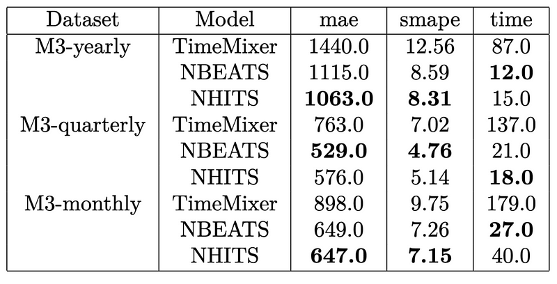
From the table above, we can see that NHITS achieves the top performance overall.
Also, TimeMixer definitely takes the longest to run, being about seven times slower than the fastest model. Furthermore, it is far from achieving competitive error metrics when compared to NHITS and N-BEATS.
It seems that the performance of TimeMixer on for short horizon forecasting is underwhelming, so let’s test it for longer horizons.
Forecasting on a long horizon
The setup is similar for running the model on the ETT dataset.
Again, we define a function to load the dataset, its validation size, test size, and frequency.
def load_data(name):
    if name == 'Ettm1':
        Y_df, *_ = LongHorizon.load(directory='./', group='ETTm1')
        Y_df['ds'] = pd.to_datetime(Y_df['ds'])
        freq = '15T'
        h = 96
        val_size = 11520
        test_size = 11520
    elif name == 'Ettm2':
        Y_df, *_ = LongHorizon.load(directory='./', group='ETTm2')
        Y_df['ds'] = pd.to_datetime(Y_df['ds'])
        freq = '15T'
        h = 96
        val_size = 11520
        test_size = 11520

    return Y_df, h, val_size, test_size, freq
Here, we test TimeMixer against PatchTST and iTransformer, as they usually perform best on long-horizon forecasting.
Specifically, we test on a horizon of 96 time steps.
For this experiment, we run cross-validation to have a more robust assessment of the each model’s performance. We also use the optimal parameters as reported by their respective papers.
DATASETS = ['Ettm1', 'Ettm2']

for dataset in DATASETS:

    Y_df, horizon, val_size, test_size, freq = load_data(dataset)

    timemixer_model = TimeMixer(input_size=horizon,
                                h=horizon,
                                n_series=7,
                                e_layers=2,
                                d_model=16,
                                d_ff=32,
                                down_sampling_layers=3,
                                down_sampling_window=2,
                                learning_rate=0.01,
                                scaler_type='robust',
                                batch_size=16,
                                early_stop_patience_steps=5)

    patchtst_model = PatchTST(input_size=horizon,
                              h=horizon,
                              encoder_layers=3,
                              n_heads=4,
                              hidden_size=16,
                              dropout=0.3,
                              patch_len=16,
                              stride=8,
                              scaler_type='identity',
                              max_steps=1000,
                              early_stop_patience_steps=5)

    iTransformer_model = iTransformer(input_size=horizon,
                                      h=horizon,
                                      n_series=7,
                                      e_layers=2,
                                      hidden_size=128,
                                      d_ff=128,
                                      scaler_type='identity',
                                      max_steps=1000,
                                      early_stop_patience_steps=3)

    models = [timemixer_model, patchtst_model, iTransformer_model]

    nf = NeuralForecast(models=models, freq=freq)

    nf_preds = nf.cross_validation(df=Y_df, val_size=val_size, test_size=test_size, n_windows=None)
    nf_preds = nf_preds.reset_index()

    evaluation = evaluate(df=nf_preds, metrics=[mae, mse], models=['TimeMixer', 'PatchTST', 'iTransformer'])
    evaluation.to_csv(f'{dataset}_results.csv', index=False, header=True)
To evaluate the performance of these models, we use the mean absolute error (MAE) and mean squared error (MSE) as they are typically used for these benchmarks.
Note that the metrics are averaged for the prediction of all seven series in both ETTm1 and ETTm2 datasets.
The results of this experiment are shown below.
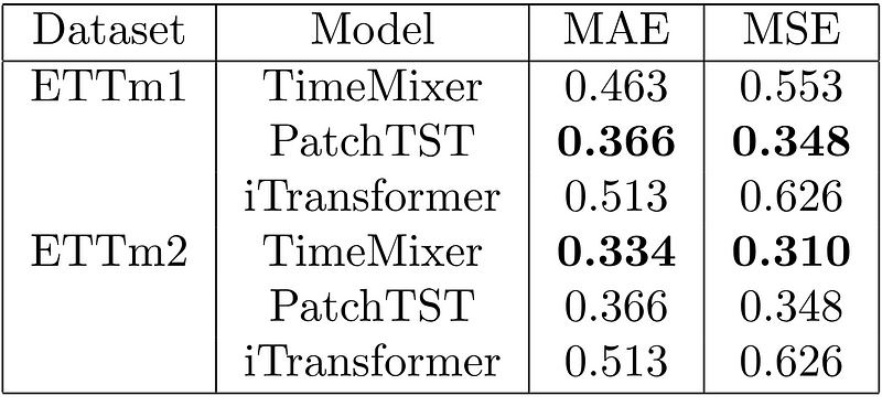
From the table above, we can see that PatchTST achieves the best result for ETTm1, while TimeMixer gets the top place for ETTm2.
Of course, this is not a comprehensive benchmark, but it is interesting to see TimeMixer perform much better in forecasting longer horizons than shorter horizons.
Therefore, if you are forecasting more than one seasonal period, TimeMixer should be considered in your tests.
Conclusion
TimeMixer is an MLP-based model that uses feature mixing at different scales to capture both micro and macro variations in time series and make predictions.
In our small benchmark, we noticed that TimeMixer is not suitable for short-horizon forecasting, as it does not perform better than NHITS or N-BEATS, and it is much slower than the latter.
However, for long-horizon forecasting, TimeMixer achieved very good results, and it was the top performing model for the ETTm2 dataset when compared to iTransformer and PatchTST.
Now, these benchmarks are far from being comprehensive, and they were meant to teach how to use the model in Python, and see it in action.
As always, I believe that each problem requires its own unique solution, so make sure to test TimeMixer and other models to find the optimal model for your specific scenario.
Thanks for reading! I hope that you enjoyed it and that you learned something new!
Learn the latest time series analysis techniques with my free time series cheat sheet in Python! Get the implementation of statistical and deep learning techniques, all in Python and TensorFlow!
Cheers 🍻
Support me
Enjoying my work? Show your support with Buy me a coffee, a simple way for you to encourage me, and I get to enjoy a cup of coffee! If you feel like it, just click the button below 👇

References
S. Wang et al., “TimeMixer: Decomposable Multisclae Mixing For Time Series Forecasting.” Accessed: Jul. 19, 2024. [Online]. Available: https://arxiv.org/pdf/2405.14616
Original code repository of TimeMixer: GitHub
Stay connected with news and updates!
Join the mailing list to receive the latest articles, course announcements, and VIP invitations!
Don't worry, your information will not be shared.
I don't have the time to spam you and I'll never sell your information to anyone.
