Time-MoE: The Latest Foundation Forecasting Model

Traditionally, the field of time series forecasting relied on data-specific models, where a model was trained on a specific dataset and task. If the data or the forecast horizon changed, the model also had to be changed.

Since October 2023, researchers have been actively developing foundation forecasting models. With these large time models, a single model can now handle different forecasting tasks from different domains, at different frequencies, and with virtually any forecast horizon.

Such large time models include: 

• TimeGPT, which is accessed via API making it easy to perform forecasting, fine-tuning without using local resources
• Lag-Llama, an open-source model for probabilistic forecasting that constructs features from lagged values
• Chronos, a model based on T5 that translated the unbounded time series domain to the bounded language domain through tokenization and quantization
• Moirai, a model that supports exogenous features and the first to publicly share their dataset LOTSA containing more than 27B data points. 

To the list above, we can also add TinyTimeMixers and TimesFM. We have also seen large language models (LLMs) being reprogrammed for time series forecasting with Time-LLM. 

In October 2024, another large time model is proposed: Time-MoE. In the paper Time-Moe: Billion-Scale Time Series Foundation Models With Mixture of Experts, researchers proposed a new foundation model that leverages a mixture of experts architecture, just like RMoK, and they also published publicly the largest open-source time series dataset to date containing 300B data points. 

In this article, we explore in detail the architecture behind Time-MoE, as well as its pretraining protocol, a crucial aspect when analyzing large time models as it set their forecasting capabilities.

Then, we conclude the article with a hands-on experiment where we apply Time-MoE in a forecasting project and compare its performance to other data-specific models, like NHITS and TSMixer.

For more details on Time-MoE, make sure to read the original paper.

Let’s get started!

Discover Time-MoE

Time-MoE, where MoE stands for mixture of experts, is an open-source foundation forecasting model. It is a decoder-only model that uses channel independence, meaning that if multiple series are passed to the model, the model will forecast them separately, as univariate series.

Below, we can see an illustration of its architecture.

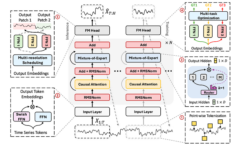
From the figure above, and also from its name, we can see that the model leverages the mixture-of-experts structure, which can route inputs to different specialized networks within the model. 

Starting at the bottom of the figure, we can see that the input series is first tokenized into a sequence of data points and mapped to an embedding. Then, the data is processed by a causal multi-head self-attention mechanism followed by the mixture-of-expert layers. The final step is then to process the data through feed-forward networks, which are optimized to forecast at different horizons.

There is of course a lot more to unpack, so let’s take a look at each step in more detail.

Tokenization and embedding

As mentioned before, the first step is to tokenize and embed the input series. 

Here, a simple point-wise tokenization method is used, meaning that point is its own token.

This differs from other foundation models, like Moirai and TimesFM where the series is first patched and then tokenized, meaning that groups of data points are tokenized together. 

This was shown to improve the forecasting performance, as the model can learn local relationships with neighboring data points. Also, it reduces the memory and computation requirements, since fewer tokens need to be processed.

On the other hand, by tokenizing each point individually, the model remains flexible in treating sequences of any arbitrary length, without having to use padding.

Once the series is tokenized and embedded, it is sent to the Transformer backbone.

Mixture-of-expert Transformer backbone

Inside the mixture-of-expert Transformer backbone is where the model learns different relationships and patterns in the input series. 

First, input is normalized using a root mean squared layer. In this step, we simply divide each element by the root of the mean of the square of each element, as shown in the equation below.

By normalizing the data, we enhance the model’s training stability and reduce the computational overhead.

Then, the data is processed by a causal self-attention mechanism. Causal attention is especially critical for time series forecasting, as it prevents the model from looking into the future, meaning that each prediction is only based on the known outputs at previous positions.

After, the data enters the mixture-of-expert layer, which is illustrated below.

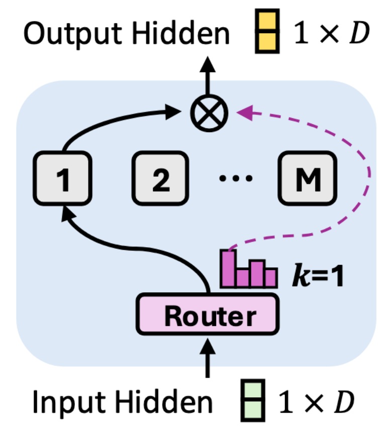
There, a router, or a gating network, decides which expert network is more appropriate to process any individual time series point. 

Here, the expert network is a simple feed-forward network. While they share the same architecture, each expert will specialize in different patterns and relationships. 

A single time point can be routed to a one or multiple experts. If a point passes through multiple experts, the results are combined through a weighted sum. 

Although not illustrated above, there is also a shared expert in the layer that sees all data points. This helps capture information across the entire time series.

As an analogy, we can think of this mixture-of-experts layer as a medical center. We have specialized doctors (individual experts) that excel at very specific uses cases. We have general practitioners (shared expert) who see all types of cases. A patient (a data point) sees the general practitioner and can then be sent to either one or multiple specialists.

This entire backbone composed of normalization, causal self-attention and mixture-of-experts layers represents a single layer. This layer is duplicated many times, allowing the model to capture a wide array of patterns in the data.

Once the data is processed by the backbone, it reaches the forecasting head.

Multi-resolution forecasting

Here, Time-MoE introduce multi-resolution forecasting, which allows the model to predict at different scales simultaneously.

In practice, this is done by training multiple feed-forward networks to specialize in forecasting different horizons, as shown below.

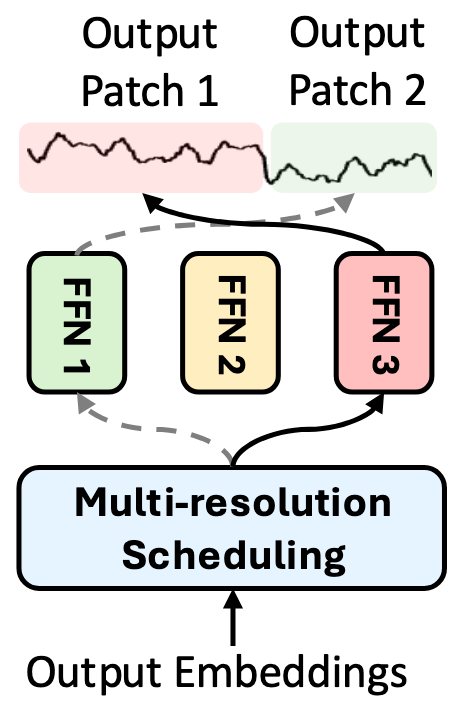
Each head illustrated above is responsible for predicting specific horizons. For example, FFN 1 can specialize in forecasting the next time step, FFN 2 is optimized to forecast the next 7 time steps, and FFN 3 can forecast the next 30 time steps.

At the time of inference, we schedule each head such as to minimize the number of passes needed.

For example, if a user wants to forecast on a horizon of 8, then we make a pass through FFN 2 (h=7), and FFN 1 (h=1). This means that the model internally forecasts the next 7 time steps, then the next time step, resulting in a predicted sequence of 8 time steps, and requiring only two passes.

That way, Time-MoE can handle any arbitrary forecasting horizons, since the forecasting head has many feedforward networks that output either long or short horizon sequences.

Now that we have a deep understanding of the inner workings of Time-MoE, let’s explore its pretraining protocol and the data that was used.

Pretraining Time-MoE

One of the greatest challenges in pretraining large time models is in accessing large volumes of high-quality open-source data.

To that end, the researchers behind Time-MoE curated Time-300B (available on HuggingFace), which is the largest time series dataset publicly available totaling 300B data points.

This dataset is composed of series from various domains, such as energy, finance, healthcare, nature, sales, and more. Around 3% of the dataset is composed of synthetic data that was used to further expand the diversity and quantity of the dataset. 

Data in Time-300B contains series at different frequency, from the second-level to the yearly frequency, which is crucial in building foundation forecasting models that are adaptable to different scenarios.

Time-MoE configurations

The model is available in three different sizes, as summarized in the table below.

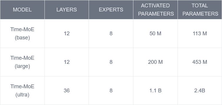
In the table above, note that the layers correspond to the number mixture-of-expert Transformer backbones are in the model. Notice also that all models use 8 experts. Finally, the activated parameters are those that are trained in the model, while other parameters are held constant.

At the time of writing this article, only the base and large versions are available on HuggingFace.

All in all, Time-MoE looks like a promising foundation model, especially since it was trained on such a large and diverse dataset. Thus, let’s see it in action in our own small experiment.

Forecasting with Time-MoE

In this section, we will use Time-MoE in a small forecasting project, where we forecast the daily views of a blogging website. 

This dataset was compiled by myself on my own data, and it is publicly available on GitHub. The dataset is visualized below.

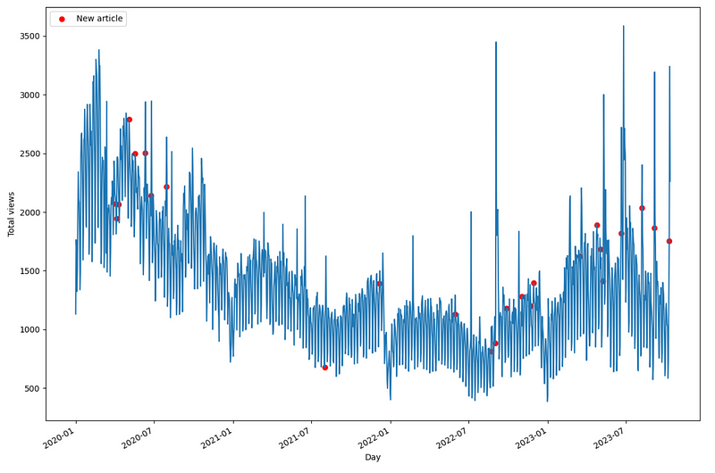
In the figure above, each red dot mark the day where a new article was published. The dataset also contains information on public holidays. However, since Time-MoE is a univariate model, those exogenous features will not be used for forecasting.

For this experiment, we use both available configurations of Time-MoE, and comapre its performance to data-specific models like NHITS and TSMixer.

The code of this experiment is entirely reproducible and available on GitHub.

Let’s get started!

Initial setup

We start off by importing the required packages. Note that we use neuralforecast for the implementations of NHITS and TSMixer.

To use Time-MoE, make sure to install transformers==4.40.1 . 

import os

import pandas as pd
import numpy as np
import matplotlib.pyplot as plt

import torch
from transformers import AutoModelForCausalLM

from neuralforecast.core import NeuralForecast
from neuralforecast.models import NHITS, TSMixer

from utilsforecast.losses import *
from utilsforecast.evaluation import evaluate

import warnings
warnings.filterwarnings("ignore")

os.environ["NIXTLA_ID_AS_COL"] = "true"
pd.set_option('display.precision', 3)

Then, we read in the dataset using pandas .

df = pd.read_csv('data/medium_views_published_holidays.csv')
df['ds'] = pd.to_datetime(df['ds'])

At this point, we are ready to make forecasts with Time-MoE.

Forecast with Time-MoE

To make it easier, we define a function that performs forecasting with a sliding window over a test set. 

def timemoe_forecast(
    df,
    target_column,
    context_length,
    prediction_length,
    test_size,
    model_size='50M',
    device = 'cpu'
):
    data = torch.tensor(df[target_column].values, dtype=torch.float32)
    
    model = AutoModelForCausalLM.from_pretrained(
        f'Maple728/TimeMoE-{model_size}',
        device_map=device,
        trust_remote_code=True
    )
    
    all_predictions = []
    
    with torch.no_grad():
        for i in range(0, test_size - prediction_length + 1, prediction_length):
            # Get sequence for current window
            start_idx = len(data) - test_size + i - context_length
            sequence = data[start_idx:start_idx + context_length]
            sequence = sequence.unsqueeze(0)  # Add batch dimension
            
            # Normalize sequence
            mean = sequence.mean(dim=-1, keepdim=True)
            std = sequence.std(dim=-1, keepdim=True)
            normalized_sequence = (sequence - mean) / std
            
            # Generate forecast
            output = model.generate(
                normalized_sequence, 
                max_new_tokens=prediction_length
            )
            
            # Denormalize predictions
            normed_preds = output[:, -prediction_length:]
            predictions = normed_preds * std + mean
            all_predictions.append(predictions.squeeze(0))
    
    return torch.cat(all_predictions).numpy()

In the function above, we can pass a DataFrame and specify our target column, the length of the input sequence, the length of the prediction, the size of the test set, the model size and the device on which we are forecasting.

Time-MoE is initialized using AutoModelForCausalLM and the data is transformed to tensors.

Then, for each window in the test set, the data is normalized and sent to Time-MoE. The predictions are then denormalized and we concatenate everything to get a single sequence of predictions.

Note that Time-MoE expects the input data to be normalized and to have a shape of (batch, input_length).

For this particular scenario, we use a horizon of 7 days and an input sequenc of six times the horizon (6 x 7 = 42). The last 168 time steps are reserved for the test set. 

Thus, we can then run our function:

h = 7

timemoe_preds_50M = timemoe_forecast(
    df=df,
    target_column='y',
    context_length=6*h,
    prediction_length=h,
    test_size=168,
    device='cpu'
)

Then, we store the predictions in a DataFrame for evaluation later on.

preds_df = df[-168:]
preds_df['Time-MOE'] = timemoe_preds_50M

We can also optionally plot the predictions as shown below.

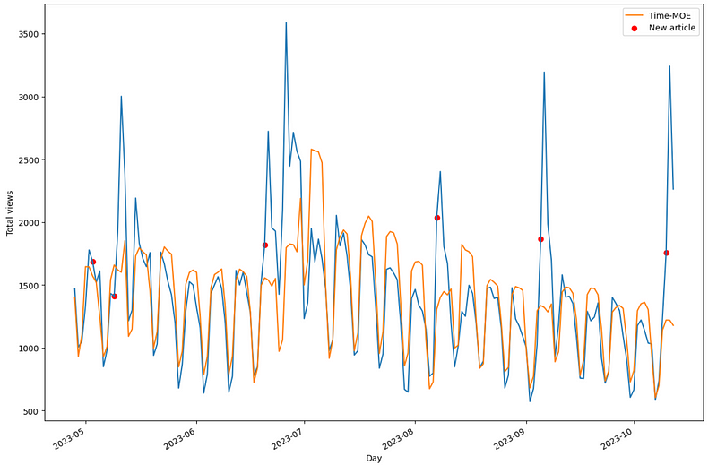
From the figure above, we can see that Time-MoE does a great job at forecasting the overall trend and seasonality of the data, but it misses the very large peaks that occur after an article is published. This makes sense as the model does not support exogenous features.

Then, let’s also forecast using the larger model for comparison.

timemoe_preds_200M = timemoe_forecast(
    df=df,
    target_column='y',
    context_length=6*h,
    prediction_length=h,
    test_size=168,
    model_size='200M',
    device='cpu'
)

preds_df['Time-MOE-200M'] = timemoe_preds_200M

Once this is done, let’s then train data-specific models for this scenario.

Training NHITS and TSMixer

As a comparison, let’s now train two data-specific models for our current dataset: NHITS and TSMixer.

models = [NHITS(h=h,
                input_size=5*h,
                max_steps=1000,
                early_stop_patience_steps=3,),
          TSMixer(h=h,
                  input_size=5*h,
                  n_series=1,
                  max_steps=1000,
                  early_stop_patience_steps=3)]

Then, using neuralforecastwe can initialize the NeuralForecast object and run cross-validation. Note that we do not pass the exogenous features for a fair evaluation against Time-MoE.

nf = NeuralForecast(models=models, freq='D')

cv_df = nf.cross_validation(
    df=df,
    step_size=h,
    val_size=168,
    test_size=168,
    n_windows=None
)

Evaluation

At this point, we have predictions from Time-MoE, NHITS and TSMixer. We are then ready to evaluate the performance of each method.

Here, we measure both the mean absolute error (MAE) and symmetric mean absolute percentage error (sMAPE) using utilsforecast.

cv_df = cv_df.drop(['ds', 'cutoff'], axis=1)

evaluation = evaluate(
    cv_df,
    metrics=[mae, smape],
    target_col='y',
    id_col='unique_id'
)

The evaluation table and bar plots of the metrics are shown below.

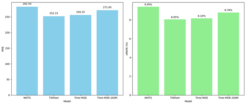
From the figures above, we first notice that the base version of Time-MoE performs better than its larger counterpart. This is interesting, as larger foundation models tend to perform better. 

However, we are only testing on a single dataset, so it might be that it just happens that the smallest version performs best in this case.

We also notice that Time-MoE performs better than NHITS, even though it was specifically trained on this dataset. Yet, TSMixer achieved the lowest MAE and sMAPE, meaning that it is the champion model. Nevertheless, it only outperforms Time-MoE by a slight margin.

My opinion on Time-MoE

Time-MoE is has suprised me on multiple fronts. It is actually one of the easiest open-source model to use with a very straightforward setup.

While Lag-Llama requires you to clone the repo, or Moirai and Chronos rely on GluonTS, Time-MoE basically only needs the transformers library to be used.

Since it relies on the transformers library, the logic of making predictions is relatively simple and easy to adapt, just like we did for predicting with sliding windows over a test set.

Also, the fact that the researchers open-sourced their entire dataset with more than 300B is an amazing contribution to the scientific community and it will definitely drive more work and research in large time models.

Still, at the time of writing, there are some shortcomings to the Time-MoE:

• it only supports univariate forecasting
• cannot use exogenous features
• The largest version is not on HuggingFace (yet)
• There are no instructions for fine-tuning (yet)
• We must normalize the data manually

Still, in our small experiment, the model is performant and faster to use than training our own model from scratch. However, there is still a trade-off, whereas TSMixer took longer to train and predict, it also resulted in the best performance.

Conclusion

Time-MoE is a decoder-only large time model that uses the mixture-of-experts architecture to perform zero-shot univariate forecasting.

The model is still being actively worked on, meaning that we do not have support for exogenous features, and there are no fine-tuning instructions.

However, in our small experiment, we experienced how easy it is to use Time-MoE, and it gives suprisingly good results, even when compared to data-specific models.

Of course, a single experiment is not indicative of the true performance of any single model. Make sure to test Time-MoE and other methods for your specific scenario.

Thanks for reading! I hope that you enjoyed it and that you learned something new!

Learn the latest time series analysis techniques with my free time series cheat sheet in Python! Get the implementation of statistical and deep learning techniques, all in Python and TensorFlow!

Cheers 🍻

Support me

Enjoying my work? Show your support with Buy me a coffee, a simple way for you to encourage me, and I get to enjoy a cup of coffee! If you feel like it, just click the button below 👇

References

[1] X. Shi et al., “Time-MoE: Billion-Scale Time Series Foundation Models with Mixture of Experts,” arXiv.org, 2024. https://arxiv.org/abs/2409.16040 (accessed Oct. 27, 2024).

[2] Official repository of Time-MoE — GitHub

[3] Time-300B dataset available on HuggingFace — HuggingFace