The Complete Introduction to Time Series Classification in Python
Jan 13, 2025
Photo by Jordan Whitt on Unsplash
Time series data is omnipresent in many industries, and while forecasting time series is widely addressed, classifying time series data is often overlooked.
In this article, we get a complete introduction to the field of time series classification, exploring its real-life applications, getting an overview of the different methods and applying some of them in a small classification project using Python.
Let’s get started!
Defining time series classification
Time series classification is a field of supervised machine learning where one or more features are measured across time and used to assign a category.
Therefore, the goal in classifying time series is to assign a label rather than predict the future value of the series.
Use cases for time series classification
Time series classification is mostly used with sensor data. Hence, we can perform predictive maintenance and monitor different equipment to predict if a failure is likely to occur.
It is also a technique used in healthcare, such as analyzing the electrocardiogram (ECG) data. The recorded pattern can be analyzed by a model to determine if a patient is healthy or not.
Furthermore, time series classification is used for speech recognition. Spoken words can be captured as a sound wave over time, and time series classification models can be used to determine what words were spoken, and also identify the speaker.
Another application is in food spectroscopy, where a classification model is applied to the spectroscopy data to determine the alcohol content of a beverage, or identify different components of food products.
Finally, it is used in cybersecurity, where a model can identify patterns of abnormal activity, signalling a potential fraud or a breach.
As we can see, the applications of time series classification are significant in many fields and industries, making it an indispensable tool to have for any data scientist.
Overview of time series classification models
There are many different approaches to time series classification. In this section, we get an overview of each method, providing a broad explanation of their inner workings, and listing the main models.
For a more detailed breakdown of each method, including how they work and their speed of inference, consult this guide on time series classification.
Distance-based models
These models rely on a distance metric to classify samples. The most common metric is the Euclidean distance.
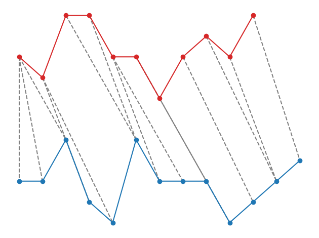
Dynamic time warping (DTW) is a more robust distance measure, as it finds the optimal match between each point of two series, allowing it to handle series of different lengths and recognize patterns that are slightly out of phase, as shown below.
Distance-based models include:
- K-nearest neighbors (KNN)
- ShapeDTW
Dictionary-based models
These models encode patterns in the series using symbols, and then use the frequency of occurrence of each symbol to classify time series.
Dictionary-based models include:
- BOSS
- WEASEL
- TDE
- MUSE
Ensemble methods
These methods are not models, but rather protocols used with other estimators.
Basically, it involves taking multiple base estimators and combining their prediction to get a final prediction.
The main advantage of ensemble method, is that it can take a univariate model and apply it on a multivariate dataset.
With the bagging technique, a univariate model can be trained on each feature of a dataset, and we can then combine the prediction from all estimators, effectively using information from all features.
Methods include:
- Bagging
- Weighted ensemble
- Time series forest
Feature-based methods
Once again, this group represents methods and not models to extract different features from time series. These features are then used to train any arbitrary machine learning model for classification.
Feature-based methods include:
- Summary features (min, max, mean, median, etc.)
- Catch22
- Matrix profile
- TSFresh
Interval-based models
These models extract multiple intervals from time series and compute features, using the methods listed above. These features are then used to train a classifier.
Such models include:
- RISE
- CIF
- DrCIF
Kernel-based models
With kernel-based models, a kernel function is applied to map the current series to another dimensional space where it would technically be easier to classify.
Common kernels include the RBF kernel and the convolutional kernel.
Example models are:
- Support vector classifier (SVC)
- Rocket
- Arsenal (an ensemble of Rocket)
Shapelet classifier
A shapelet classifier relies on extracting shapelets: the most discriminative subsequences of a time series.
The distance between the shapelet and a particular series is then used for classification.
Meta classifier
Finally, the meta classifier combines different methods listed above to ensemble them and produce a robust classifier that can used with virtually any series and result in good performance.
HIVE-COTE is an example of a meta classifier that combines TDE, Shapelet, DrCIF and Arsenal.
While this model looks like a universal solution to classification, it is very slow to train, and other methods are worth testing before resorting to HIVE-COTE.
As you can see, there is a vast array of methods for time series classification. Some are faster than others, some handle only univariate data.
Knowing each method’s strength and inner workings is key in building the best classification model for your particular scenario. However, a deep dive into each method is outside the scope of this article, as this is meant to give an introduction to classification and get you some hands-on experience.
As such, let’s apply some classification models in a small project using Python.
Hands-on time series classification project
In this section, we apply some techniques listed above to a classification task.
Here, we use the BasicMotions dataset, donated by Jack Clements to the UEA archive and publicly accessible here through the GPL license.
This dataset compiles data from four students wearing a smartwatch and performing different activities: standing, walking, running and playing badminton.
The watch has an accelerometer and a gyroscope that recorded data in three different axes (x, y, z), resulting in six features in total. However, the dataset is rather small with only 40 training and testing samples.
The objective is then to classify the activity being performed from the data collected by the accelerometer and gyroscope. Here, we implement the K-nearest neighbor algorithm and use bagging along with WEASEL to see which approach performs best.
The full source code is available on GitHub.
Initial setup
First, we import the required packages for time series classification.
For this task, I think that sktime is the best option, as it implements a comprehensive list of classification method through a familiar interface that mimics scikit-learn. It also plays very well with scikit-learn making it easy to evaluate our models and use other machine learning models for time series classification.
import pandas as pd
import numpy as np
import matplotlib.pyplot as plt

from sktime.datasets import load_basic_motions
from sklearn.model_selection import GridSearchCV, KFold
Then, we read the dataset. Since this is a common dataset to get started with time series classification, it is also available through the sktime package.
X_train, y_train = load_basic_motions(split='train', return_type='numpy3D')
X_test, y_test = load_basic_motions(split='test', return_type='numpy3D')
Notice that we specify return_type='numpy3D’. This is the most flexible data format for time series classification.
We can print out the shape of X_train and get (40, 6, 100). The shape corresponds to (num_samples, num_features, num_timesteps). Thus, we see that X_train has:
- 40 samples
- 6 features
- Each feature is measured across 100 time steps
Then, we can visualize our data to see the difference in patterns between each activity. Below, we show the difference between walking and playing badminton.
series_indices = [0, 10, 20, 30]
categories = ['standing', 'running', 'walking', 'badminton']
features = ["accel_1", "accel_2", "accel_3", "gyro_1", "gyro_2", "gyro_3"]

selected_series = X_train[series_indices]

fig, axes = plt.subplots(4, 1, figsize=(10, 18))

for i in range(4):
    for j in range(selected_series.shape[1]):
        axes[i].plot(selected_series[i, j], label=features[j])

    axes[i].set_title(f"Category: {categories[i]}")
    axes[i].set_xlabel("Time Steps")
    axes[i].set_ylabel("Values")
    axes[i].legend()

plt.tight_layout()
plt.show()
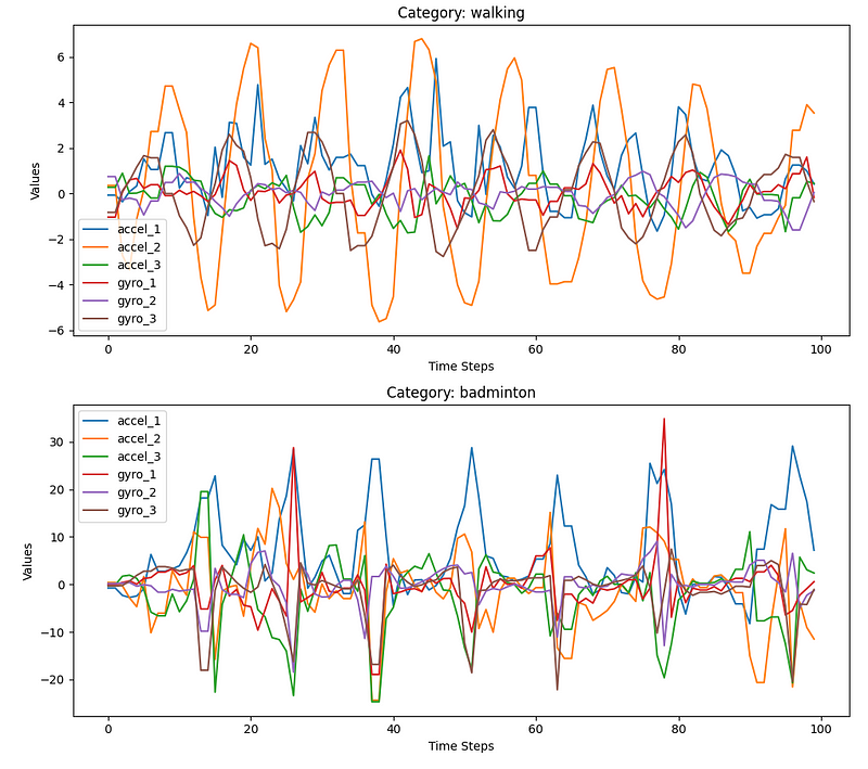
In the figure above, we can see very clear patterns for each activity. For example, the accelerator displays short bursts when a person is playing badminton, something we do not observe during walking.
The idea is now to feed those features measured across time to a machine learning model and see if it can correctly classify each activity.
Classification with KNN
One of the simplest methods we can use is a distance-based model like K-nearest neighbors (KNN).
Again, this method uses a distance metric, like the Euclidean distance or dynamic time warping (DTW), and assigns the label of the sample that has the shortest distance to a given series.
Thus, as a small experiment, let’s tune KNN to determine which distance metric is best to use between Euclidean and DTW.
from sktime.classification.distance_based import KNeighborsTimeSeriesClassifier

knn = KNeighborsTimeSeriesClassifier(n_neighbors=1)

params = {
    "distance": ['euclidean', 'dtw']
}
tuned_knn = GridSearchCV(
    knn,
    params,
    cv=KFold(n_splits=5)
)
tuned_knn.fit(X_train, y_train)
y_pred_knn = tuned_clf.predict(X_test)

print(tuned_knn.best_params_)
Here, the best distance metric to use is DTW, and we already made predictions using this optimal configuration.
Classification with bagging and WEASEL
Next, let’s use bagging along with WEASEL to classify our dataset.
WEASEL is a dictionary-based model, meaning that it encodes patterns with bag-of-words.
For example, an increasing trend might be encoded as “aaa” while a decreasing trend can be encoded as “aab”. The frequency of these bag-of-words is then used to train a model and make predictions.
However, WEASEL is a univariate model, meaning that it can only process a single feature. Since our datasethas six features, the model might miss important information resulting in poor performances.
To solve that, we can use bagging. With this technique, we can train multiple base estimators and combine them to get a final prediction.
In this case specifically, we can train six different WEASEL models that will specialize in each feature. We can then combine the predictions of all individual models to get the final label.
from sktime.classification.ensemble import BaggingClassifier
from sktime.classification.dictionary_based import WEASEL
from sklearn.preprocessing import LabelEncoder

encoder = LabelEncoder()
encoder.fit(y_train)
y_train_encoded = encoder.transform(y_train)

base_clf = WEASEL(alphabet_size=3,support_probabilities=True, random_state=42)

clf = BaggingClassifier(
    base_clf,
    n_estimators=6, # there are 6 features in total
    n_features=1,
    random_state=42
)
clf.fit(X_train, y_train)
y_pred_bagging = clf.predict(X_test)
y_pred_bagging = encoder.inverse_transform(y_pred_bagging)
In the code block above, we first label encode our target, as it is a requirement for using bagging.
Then, notice that we specify alphabet_size=3. This determines how many letters can go in the bag-of-words to encode patterns. A larger alphabet can encode more complicated patterns, but using a value of 3 is a reasonable starting point.
Also, when used with bagging, we must set support_probabilities=True. The probabilities of each individual model are then combined to get the final prediction.
Once the base estimator is defined, we initialize the BaggingClassifier and specify n_estimators=6, since there are six features in the dataset and each estimator will consider n_features=1.
Using this method, we have successfully applied a univariate model on a multivariate dataset and used all the information to perform classification.
Evaluation
Having used two different approaches for classification, let’s evaluate both of them to see which performs best.
We can display the classification report to get a breakdown of the performance for each class.
from sklearn.metrics import classification_report, f1_score

knn_report = classification_report(y_test, y_pred_knn, zero_division=0.0)
bagging_report = classification_report(y_test, y_pred_bagging)
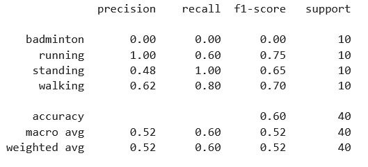
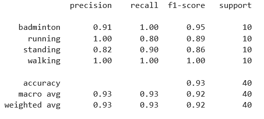
Looking at both reports above, we notice that the KNN model completely fails to predict the badminton class, resulting in an overall poor performance.
However, bagging with WEASEL yields very good results, as it perfectly labels the walking activity and achieves a F1-score of 0.92.
We can optionally visualize both F1-scores in the figure below.
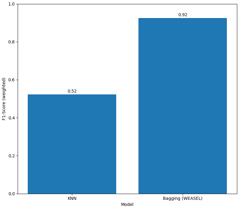
Once again, from the figure above, we can see that bagging with WEASEL yields the best results, with a F1-score of 0.92.
Thus, it is interesting to see the benefits of using bagging with a univariate model, allowing it to capture information from all features and resulting in good performances.
Conclusion
In this article, we introduced the field of time series classification.
We discovered some of its real-life applications in healthcare, cybersecurity and predictive maintenance and got an overview of the different methods used for time series classification.
We then completed our first classification project using KNN and bagging with WEASEL. Keep in mind that this project is meant to get us started in time series classification, as there is of course much more to discover.
Thanks for reading and I hope that you learned something new!
Cheers 🍻
Next steps
To keep learning on time series classification, leave a comment or clap to let me know that you want my to cover more on the subejct.
Also, you can download my free guide on time series classification for a reference guide on all available methods, how they work, their speed of inference, and for data sources to practice time series classification.
Finally, if you are serious about mastering time series classification, check out my course: Time Series Classification in Python. This is the most complete course on the subject, covering both machine learning and deep learning methods in detail, along with guided capstone projects with real-life datasets.
Support me
Enjoying my work? Show your support with Buy me a coffee, a simple way for you to encourage me, and I get to enjoy a cup of coffee!
References
BasicMotions dataset — http://www.timeseriesclassification.com/description.php?Dataset=BasicMotions
Sktime — https://www.sktime.net/en/stable/
Stay connected with news and updates!
Join the mailing list to receive the latest articles, course announcements, and VIP invitations!
Don't worry, your information will not be shared.
I don't have the time to spam you and I'll never sell your information to anyone.

