SOFTS: The Latest Innovation in Time Series Forecasting

In recent years, deep learning has been successfully applied for time series forecasting, where new architectures have incrementally set new standards for state-of-the-art performances.

It all started with N-BEATS in 2020, which was followed by NHITS in 2022. In 2023, PatchTST and TSMixer were proposed, and they still rank among the top forecasting models. 

More recently, we discovered the iTransformer, which further pushed the performance of deep learning forecasting models.

Now, we introduce the Series-cOre Fused Time Series forecaster or SOFTS. 

Proposed in April 2024 in the article SOFTS: Efficient Multivariate Time Series Forecasting with Series-Core Fusion, this model employs a centralized strategy for learning interactions across different series, resulting in state-of-the-art performances in multivariate forecasting tasks.

In this article, we explore the architecture of SOFTS in detail, and discover the novel STar Aggregate-Dispatch (STAD) module which is responsible for learning interactions between time series. Then, we apply this model in a univariate and multivariate forecasting scenario.

For more details, make sure to read the original paper.

Learn the latest time series forecasting techniques with my free time series cheat sheet in Python! Get the implementation of statistical and deep learning techniques, all in Python and TensorFlow!

Let’s get started!

Discover SOFTS

As mentioned above, SOFTS stands for Series-cOre Fused Time Series. 

The motivation behind SOFTS comes from the realization that long-horizon multivariate forecasting is crucial for decision-making, but it also poses a difficult challenge.

On one hand, we have Transformer-based models that try to reduce the complexity of the Transformer by using techniques like patch embedding and channel independence, as in PatchTST. However, with channel independence, we remove the interactions of each series on one another, so we potentially overlook predictive information.

The iTransformer partially solved that problem by embedding the entire series, as in an extreme case of patch embedding, and sending them through the attention mechanism. 

Still, Transformer-based models are computationally complex and can require more time to train on very large datasets.

On the other hand, we have MLP-based models. Those models are usually fast and produce very strong results, but their performance tend to degrade when many series are present.

With SOFTS, the researchers suggest a MLP-based coupled with the STAD module. Since the MLP is the building block of the model, it remains fast to train. As for the STAD module, it allows for learning relationships between each series, like the attention mechanism, but more computationally efficient.

Architecture of SOFTS

Below, we can see the architecture of SOFTS.

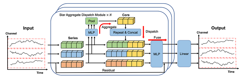
In the figure above, we first see that each series is embedded individually, just like in iTransformer. 

The embeddings are then sent to the STAD module. There, interactions between each series are centralized and learned, before being dispatched back to the individual series and fused together.

A final linear layer then produces the forecasts.

There is a lot to dissect from this architecture, so let’s explore each component in more detail.

Normalization and embedding

First, normalization is used to calibrate the distribution of the input series. Specifically, reversible instance normalization, or RevIn, is used.In short, it centers the data around a mean of zero with a unit variance. 

Then, each series is embedded separately, in an extreme case of patching, just like in the iTransformer model. 

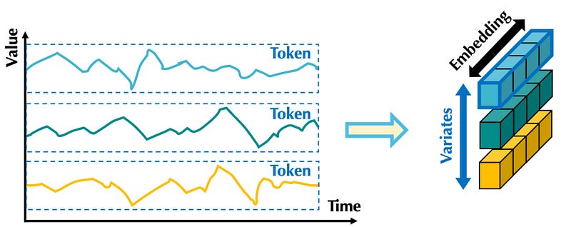
In the figure above, we can see that embedding the entire series is like applying patch embedding where the patch length equals the length of the input series.

That way, the embedding contains information of the entire series across all time steps.

The embedded series are then sent to the STAD module.

STar Aggregate-Dispatch (STAD)

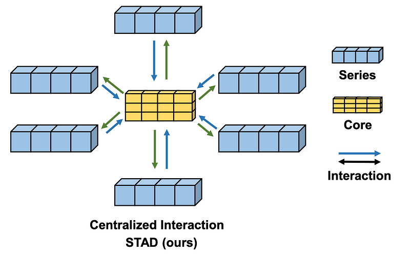
The STAD module is really what differentiates the SOFTS model from other forecasting methods. 

Here, a centralized strategy is used to find interactions between all time series. This is done through the core.

Before entering the core, the embedded series are sent through a MLP and a pooling layer. Note that stochastic pooling is used here.

Then, this learned representation is concatenated to form the core, represented by the yellow block in the figure above.

Once the core is built, we enter the repeat and concatenate step, where the core representation is dispatched to each series representations. 

Let’s bring back the image of the architecture of SOFTS to illustrate that operation.

Note that the information not captured by the MLP and pooling layers are added to the core representation through residual connections. 

Then, the core representation concatenated with the residuals of their corresponding series are all sent through a MLP layer during the fuse operation. 

Finally, a linear layer takes the output of the STAD module to generate the final forecasts for each series.

One of the main advantages of the STAD module is its reduced complexity compared to other methods for capturing channel interactions like the attention mechanism.

Here, the STAD module has a linear complexity, while the attention mechanism has a quadratic complexity, meaning that STAD can technically handle large datasets with multiple series more efficiently.

Now that we have a deeper understanding of SOFTS, let’s apply it in a small forecasting experiment, testing it in both a univariate and multivariate scenario.

Forecasting with SOFTS

In this section, we implement the SOFTS model in both a univariate and multivariate long-horizon forecasting scenario.

Here, we use the popular Electricity Transformer dataset released under the Creative Commons License.

This benchmark dataset that tracks the oil temperature of an electricity transformer from two regions in a province of China. For both regions, we have a dataset sampled at each hour and every 15 minutes, for a total of four datasets.

For this experiment in particular, we use the datasets samples at every 15 minutes.

Here, I extended the neuralforecast library with an adapted implementation of the SOFTS model from their official repository. That way, we have a streamlined experience for using and testing different forecasting models.

Note that at the time of writing this article, SOFTS is not in a stable release of neuralforecast just yet. 

To reproduce the results, you may need to clone the repository and work in this branch. 

If the branch is merged, then you can run:

pip install git+https://github.com/Nixtla/neuralforecast.git

The code for this experiment is available on GitHub. 

Let’s get started!

Initial setup

As always, we start off by importing the required packages for this experiment. Specifically, we use datasetsforecast to load the dataset in the required format for training models with neuralforecast, and we use utilsforecast to evaluate the performance of the models.

import pandas as pd
import numpy as np
import matplotlib.pyplot as plt

from datasetsforecast.long_horizon import LongHorizon

from neuralforecast.core import NeuralForecast
from neuralforecast.losses.pytorch import MAE, MSE
from neuralforecast.models import SOFTS, PatchTST, TSMixer, iTransformer

from utilsforecast.losses import mae, mse
from utilsforecast.evaluation import evaluate

Then, let’s write a function to help us load the datasets, along with their standard test sizes, validation sizes, and frequency.

def load_data(name):
    if name == "ettm1":
        Y_df, *_ = LongHorizon.load(directory='./', group='ETTm1')
        Y_df = Y_df[Y_df['unique_id'] == 'OT'] # univariate dataset
        Y_df['ds'] = pd.to_datetime(Y_df['ds'])
        val_size = 11520
        test_size = 11520
        freq = '15T'
    elif name == "ettm2":
        Y_df, *_ = LongHorizon.load(directory='./', group='ETTm2')
        Y_df['ds'] = pd.to_datetime(Y_df['ds']) 
        val_size = 11520
        test_size = 11520
        freq = '15T'

    return Y_df, val_size, test_size, freq

Now, we can let’s SOFTS for univariate forecasting on the ETTm1 dataset.

Univariate forecasting with SOFTS

First, we load the ETTm1 dataset using the function defined above. Let’s also set the forecast horizon to 96 time steps. 

Usually, more prediction lengths are tested, but let’s stick to 96 only for this portion.

Y_df, val_size, test_size, freq = load_data('ettm1')

horizon = 96

Then, we initialize the different models for this particular experiment. Here, we compare SOFTS to TSMixer, iTransformer and PatchTST.

Here, we keep the default configuration for all models. We also set the maximum number of training steps to 1000, and stop training if the validation loss does not improve after three checks.

models = [
    SOFTS(h=horizon, input_size=3*horizon, n_series=1, max_steps=1000, early_stop_patience_steps=3),
    TSMixer(h=horizon, input_size=3*horizon, n_series=1, max_steps=1000, early_stop_patience_steps=3),
    iTransformer(h=horizon, input_size=3*horizon, n_series=1, max_steps=1000, early_stop_patience_steps=3),
    PatchTST(h=horizon, input_size=3*horizon, max_steps=1000, early_stop_patience_steps=3)
]

Then, we can train the model after initializing the NeuralForecast object. Specifically, we use cross-validation to get multiple forecast windows, giving us a better assessment of each model’s performance.

nf = NeuralForecast(models=models, freq=freq)
nf_preds = nf.cross_validation(df=Y_df, val_size=val_size, test_size=test_size, n_windows=None)
nf_preds = nf_preds.reset_index()

Finally, we evaluate calculate the mean absolute error (MAE) and mean squared error (MSE) for each model. 

Note that the data was previously scaled, so the reported metrics are also scaled.

ettm1_evaluation = evaluate(df=nf_preds, metrics=[mae, mse], models=['SOFTS', 'TSMixer', 'iTransformer', 'PatchTST'])

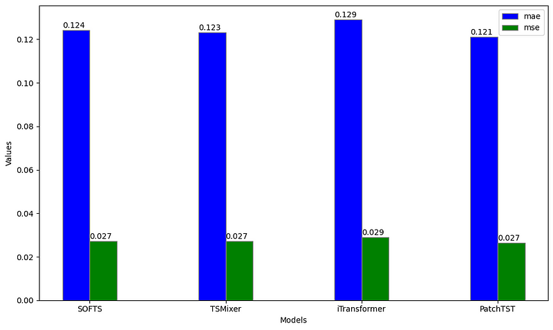
From the figure above, we can see that PatchTST achieves the lowest MAE, while SOFTS, TSMixer and PatchTST all achieve the same MSE. Thus, PatchTST remains the overall best model in this particular case.

This comes with no surprise, as PatchTST is notoriously good in this dataset, especially for univariate tasks.

Great! Now, let’s apply SOFTS in a multivariate scenario.

Multivariate forecasting with SOFTS

Using the same load_data function, we now use the ETTm2 dataset for this multivariate scenario. 

Again, we keep the forecast horizon to 96 time steps.

Y_df, val_size, test_size, freq = load_data('ettm2')

horizon = 96

Then, we simply initialize each model. Here, we only use multivariate models that learn interactions between series, so we will not use PatchTST, as it applies channel independence (meaning that each series is treated separately).

Also, notice that we keep the same hyperparameters as in the univariate scneario. We only change n_series to seven, since have seven time series interacting with each other.

models = [SOFTS(h=horizon, input_size=3*horizon, n_series=7, max_steps=1000, early_stop_patience_steps=3, scaler_type='identity', valid_loss=MAE()),
          TSMixer(h=horizon, input_size=3*horizon, n_series=7, max_steps=1000, early_stop_patience_steps=3, scaler_type='identity', valid_loss=MAE()),
          iTransformer(h=horizon, input_size=3*horizon, n_series=7, max_steps=1000, early_stop_patience_steps=3, scaler_type='identity', valid_loss=MAE())]

Now, we can train all models and make predictions. Of course, we use cross-validation to generate many forecast windows. 

nf = NeuralForecast(models=models, freq='15min')

nf_preds = nf.cross_validation(df=Y_df, val_size=val_size, test_size=test_size, n_windows=None)
nf_preds = nf_preds.reset_index()

Finally, we can evaluate the performance of each model using the MAE and MSE.

ettm2_evaluation = evaluate(df=nf_preds, metrics=[mae, mse], models=['SOFTS', 'TSMixer', 'iTransformer'])

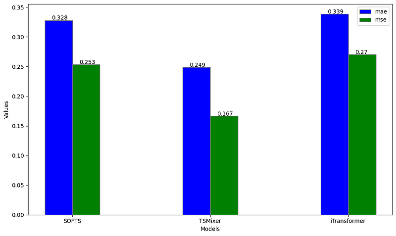
From the figure above, we notice that TSMixer larger outperforms both iTransformer and SOFTS on the ETTm2 dataset when forecasting on a horizon of 96.

While this contradicts the results from the paper, keep in mind that we did not perform hyperparameter optimization. Also, the paper reports metrics averaged over multiple forecast horizons, while we used a fixed horizon of 96 time steps.

Again, the results from this experiment may be underwhelming, but again, we did not optimize the hyperparameters and we only tested on a single dataset for a fixed forecast horizon, so this is a not a robust benchmark of the performance of SOFTS.

Conclusion

SOFTS is a promising MLP-based multivariate forecasting model that implements the novel STAD module.

The STAD module is a centralized method for learning interactions between time series that is less computationally intensive than the attention mechanism.

This results in a model capable of handling large datasets with many concurrent time series efficiently.

While the performance of SOFTS in our experiment might seem slightly underwhelming, remember that this is does not represent a robust benchmark of its performance, as we only tested on a single dataset for a fixed horizon.

As always, I believe that each problem requires its own unique solution, so make sure to test SOFTS and other models to find the optimal model for your specific scenario.

Thanks for reading! I hope that you enjoyed it and that you learned something new!

Learn the latest time series analysis techniques with my free time series cheat sheet in Python! Get the implementation of statistical and deep learning techniques, all in Python and TensorFlow!

Cheers 🍻

Support me

Enjoying my work? Show your support with Buy me a coffee, a simple way for you to encourage me, and I get to enjoy a cup of coffee! If you feel like it, just click the button below 👇

References

Lu Han, Xu-Yang Chen, Han-Jia Ye, De-Chuan Zhan. “SOFTS: Efficient Multivariate Time Series Forecasting with Series-Core Fusion”

Official implementation of SOFTS — GitHub