Kolmogorov-Arnold Networks (KANs) for Time Series Forecasting

The multilayer perceptron (MLP) is one of the foundational structures of deep learning models. It is also the building block of many state-of-the-art forecasting models, like N-BEATS, NHiTS and TSMixer.

On April 30, 2024, the paper KAN: Kolmogorov-Arnold Network was published, and it has attracted the attention of many practitioners in the field of deep learning. There, the authors propose an alternative to the MLP: the Kolmogorov-Arnold Network or KAN.

Instead of using weights and fixed activation functions, the KAN uses learnable functions that are parametrized as splines. The researchers suggest the KAN can thus be more accurate with less trainable parameters than MLPs.

In this article, we first explore splines, as they help us understand the architecture and key elements of KAN. Then, we make a deep dive inside the inner workings of KAN. Finally, we apply KAN to time series forecasting, and evaluate its performance against the standard MLP and the N-BEATS model.

For more details on KAN, make sure to read the original paper.

Learn the latest time series forecasting techniques with my free time series cheat sheet in Python! Get the implementation of statistical and deep learning techniques, all in Python and TensorFlow!

Let’s get started!

Visiting splines

Splines are at the core of the Kolmogorov-Arnold networks, so let’s take some time to understand them.

A spline is simply a function defined piecewise by polynomials. It allows us to build a smooth line crossing many data points, without resorting to using high-degree polynomials, which tend to oscillate too much. 

Consider the following example.

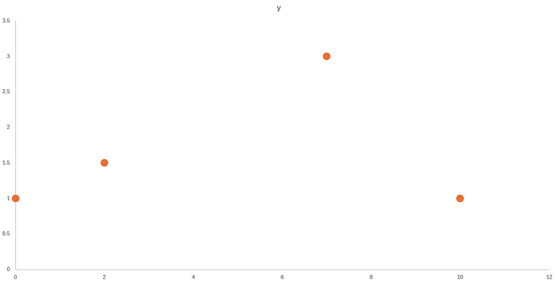
In the figure above, we can see that we have four data points. If we wish to fit a line through them, we can use a 3rd-degree polynomial. Remember that n-degree polynomials have n+1 coefficients, so we need a minimum n+1 data points to get a good fit.

We can try this out in Excel by adding a trend line to our data, and specifying a 3rd-degree polynomial.

As you can see, fitting a polynomial works well in this case, as we get a smooth curve. 

However, what happens when we have more data points?

In this case, Excel limits us to a 6th-degree polynomial, so let’s try fitting a line through seven data points as shown below.

From the figure above, the fit through the first few points is reasonable, but we get a big oscillation at the last two points on the right. This is the problem of using high degree polynomials.

In real life, we deal with very large datasets, so using increasingly large polynomials does not make sense. 

Instead, we can divide our dataset into subsequences such that we fit low-degree polynomials to each subsequence. 

In this case, instead of fitting a single line through seven data points, we could fit a 3rd-degree polynomial to the first four points, and another 3rd-degree polynomial to the last four points. Note that each set shares one data point to ensure that there is no gap in the final fit.

In the figure above, we see that we get less oscillations. However, take a close look at the fourth data point. We get a weird break in the fitted line such that it is not a smooth fit.

The point where the kink occurs is called a knot. To solve the choppiness of the curve, we add the condition that the derivatives of each polynomial must be equal at the knot. 

This ensures that a smooth fitted curve across all data points. Plus, to allow using an arbitrary amount of data points, we also set constraints on the second derivatives of each polynomial, such that the second derivatives must also be equal at the knot.

The result of splitting our data in subsequences, fitting low-degree polynomial to each sequence, and ensuring the constraints are respected at the knots gives us a spline. If the spline is composed of many 3rd-degree polynomials, we get a cubic spline.

In the figure above, we can see the result of using a spline to fit our data points. We see that the line is smooth, we do not get weird oscillations, and we can use as many points as we want.

In the case of KAN, it makes use of basis splines or B-splines. 

The idea is that any spline function can be expressed as a linear combination of B-splines. More importantly, each spline function has a unique combination of B-splines.

With all of that in mind, let’s explore the KAN architecture in more detail.

Exploring the Kolmogorov-Arnold network

Now that we have a deeper understanding of splines, let’s see how they are integrated in the architecture of Kolmogorov-Arnold networks.

First of all, the KAN is unsurprisingly based on the Kolmogorov-Arnold representation theorem. This establishes that a multivariate continuous function can be represented as a finite composition of univariate functions and the addition operation.

In simpler terms, a multivariate function boils down to combining many univariate functions.

Now, this theorem only holds practical value if the univariate functions are smooth, making them learnable. If they are non-smooth or fractal functions, they are not learnable, and so the KAN becomes useless.

Fortunately, the vast majority of use cases involve smooth functions, which is why the KAN is now proposed as an alternative to the MLP.

Architecture of KAN

Following that, the researchers built a neural network that learns univariate functions to represent a multivariate function.

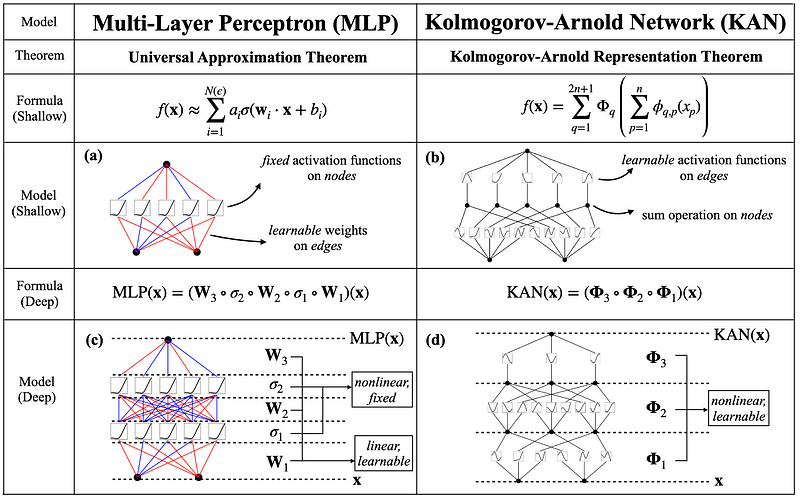
In the figure above, we see the architecture of KAN and how it compares to the MLP. 

The edges of the KAN (represented by the lines) are the learnable univariate functions, which are parametrized as B-splines. Then, at the nodes (represented as dots) a summation is performed. 

Take some time to recognize that this is the Kolmogorov-Arnold representation theorem in action as a neural network. Many univariate functions are learned and combined to ultimately represent another process.

We also see how it contrasts the MLP architecture. In the MLP, the nodes are fixed activation functions, usually a non-linear function like the rectified linear unit (ReLU). Then, at the edges, the MLP has learnable weights.

Thus, the main difference between KAN and MLP is that the non-linear functions are learnable in KAN and fixed in the MLP. Therefore, the KAN can technically better learn from the input data using less parameters, since the functions are learned and adapted according to the input data. 

Of course, with larger and deeper KANs, we get better approximation and generalization power, allowing the network to learn arbitrary functions. 

Now, the trick to making KANs deeper while remaining parameter-efficient is in grid extension.

Grid extension in KAN

Grid extension is used in KAN for each B-spline function as a method to increase the accuracy and efficiency of the model.

In the figure above, we can see the flow of activation in a KAN (left side), as well as the grid extension technique (right side) being applied to each spline.

With grid extension, we increase the granularity of the spline grid to get better approximations of complex functions. This is done by increasing the number of intervals within the same region. In the figure, this is illustrated by going from G1 = 5 to G2 = 10.

By increasing the number of intervals, we also increase the number of pieces that compose the final spline function. This in turns allows to learn more fine-grained behaviour in the data. 

This extension capability contrasts that of MLPs, where the model must be deeper in order to learn more complex functions. In KAN, this is done for each spline, so less layers are technically required to learn more complex functions.

Now that we have a good understanding of KAN and its inner workings, let’s see how we can apply it for time series forecasting using Python.

Forecasting with KAN

In this section, we test the KAN architecture on a forecasting task using Python. 

At the time of writing this article, KAN is very new, so I extended my favourite forecasting library neuralforcast with this Pytorch implementation of KAN, adapting it to time series forecasting. 

Also, it is possible that the KAN model might not be available in a stable release of neuralforecast. To reproduce the results, you can either:

• Clone the neuralforecast repository and work in this branch
• Or if the branch was merged, you can run

pip install git+https://github.com/Nixtla/neuralforecast.git

Now, for this experiment, we test the KAN model on the monthly M3 dataset made available through the Creative Commons Attribution 4.0 license.

This dataset contains 1428 unique time series, all with a monthly frequency, coming from various domains. 

The performance of KAN will be compared to that of a simple MLP and to the N-BEATS model.

All the code to reproduce these results is available on GitHub.

Let’s get started!

Initial setup

We start off by importing the required packages for this experiment.

import pandas as pd

from datasetsforecast.m3 import M3

from utilsforecast.losses import mae, smape
from utilsforecast.evaluation import evaluate

from neuralforecast import NeuralForecast
from neuralforecast.models import KAN, MLP, NBEATS

We use the datasetsforecast library to load the monthly M3 dataset in a format that is compatible with neuralforecast.

Y_df, *_ = M3.load("./data", "Monthly")

Then, we use a forecast horizon of 18, as set in the dataset specifications. We thus reserve the last 18 time steps for the test set, and use the rest of the data for training.

horizon = 18

test_df = Y_df.groupby('unique_id').tail(horizon)
train_df = Y_df.drop(test_df.index).reset_index(drop=True)

Great! At this point, we have out training and test set, so we are ready to fit our models.

Fitting models

To fit models, we simply define a list of all models we wish to train. Here, I keep their base configuration. Note that both the base KAN and MLP have only three layers: an input layer, a hidden layer, and an output layer. 

We also set a maximum of 1000 training steps, and set the patience to three, meaning that the model will stop training if the validation loss does not improve after three checks.

models = [
    KAN(input_size=2*horizon,
        h=horizon,
        scaler_type='robust',
        max_steps=1000,
        early_stop_patience_steps=3),
    MLP(input_size=2*horizon,
        h=horizon,
        scaler_type='robust',
        max_steps=1000,
        early_stop_patience_steps=3),
    NBEATS(input_size=2*horizon,
           h=horizon,
           scaler_type='robust',
           max_steps=1000,
           early_stop_patience_steps=3)
]

Awesome! Now, we create an instance of NeuralForecast which takes care of handling the data and fitting the models. Then, we call the fit method to train each model.

nf = NeuralForecast(models=models, freq='M')

nf.fit(train_df, val_size=horizon)

Once training is done, we can move on to making predictions and evaluating the performance of each model.

Evaluation

We can now take our fitted models and make predictions over the forecast horizon. Those values can then be compared to the actual values stored in the test set.

preds = nf.predict()

preds = preds.reset_index()

test_df = pd.merge(test_df, preds, 'left', ['ds', 'unique_id'])

To evaluate our models, we use the mean absolute error (MAE) and symmetric mean absolute percentage error (sMAPE). 

For this portion, we use the utilsforecast library, which conveniently comes with many metrics and utility functions to evaluate forecasting models.

evaluation = evaluate(
    test_df,
    metrics=[mae, smape],
    models=["KAN", "MLP", "NBEATS"],
    target_col="y",
)

evaluation = evaluation.drop(['unique_id'], axis=1).groupby('metric').mean().reset_index()
evaluation

The code blocks outputs the results shown below.

In the table above, we can see that KAN achieves the worst performance, even when compared to a very simple MLP. Unsurprisingly, N-BEATS achieves the best performance with a MAE of 637 and a sMAPE of 7.1%. 

While the performance of KAN is underwhelming, note that it only uses 272k learnable parameters, compared to 1.1M for the MLP and 2.2M for N-BEATS. This represents a 75% reduction in the number of parameters compared to the MLP. Nevertheless, its performance is disappointing in this scenario.

Benchmarking KAN for time series forecasting

The experiment above can easily be extended to the full M3 dataset, as well as the M4 dataset, also available through the Creative Commons Attribution 4.0 license.

The results of the benchmark as shown below. The best performance is shown in bold, and the second best is underlined.

In the table above, we can see that KAN is often the worst forecasting model, usually under-performing the simple MLP. It only beats the MLP on the weekly M4 dataset, and achieves the best performance on the hourly M4 dataset. Also notice that KAN is the slowest model in the benchmark.

For every forecasting task, the KAN is indeed more parameter-efficient than MLP or N-BEATS, but its performance is disappointing.

My opinion on KAN

The KAN architecture has attracted a lot of attention and there is a lot of hype building around the model. However, applying it to forecasting tasks generated fairly poor results.

This was a bit expected, as the MLP is not a very good forecasting model either, and the KAN is proposed as an alternative to the MLP.

Still, the authors of the paper claim better performance over the MLP, which unfortunately was not realized when applied to time series forecasting.

I believe the real potential lies in replacing MLP units by KAN in more advanced forecasting models, like N-BEATS or NHiTS. After all, time series forecasting is a challenging task, and models like the KAN and the MLP are too general to be performant by themselves. 

However, having a KAN-based N-BEATS or NHiTS can potentially make them lighter, faster and even better at forecasting, and I hope to see this being tested in the near future.

Conclusion

The Kolmogorov-Arnold network (KAN) is presented as an alternative to the foundational multilayer perceptron (MLP) in deep learning.

It applies the Kolmogorov-Arnold representation theorem stating that multivariate functions can be represented as combinations of univariate functions.

In the KAN, those univariate functions are learned and parametrized as B-splines. Contrary to the MLP which uses fixed non-linear activation functions, the splines are non-linear functions that can be learned and adapted to the training data.

This allows KAN to be more parameter-efficient than the MLP and theoretically achieve better performance.

However, applying the KAN for time series forecasting resulted in subpar performance, with the model often underperforming a very simple MLP.

Its potential probably lies in replacing the MLP in more established forecasting models, like N-BEATS or NHiTS. 

Keep in mind that KAN is very new, but it still represents an exciting advance in the field of deep learning.

Thanks for reading! I hope that you enjoyed it and that you learned something new!

Learn the latest time series analysis techniques with my free time series cheat sheet in Python! Get the implementation of statistical and deep learning techniques, all in Python and TensorFlow!

Cheers 🍻

Support me

Enjoying my work? Show your support with Buy me a coffee, a simple way for you to encourage me, and I get to enjoy a cup of coffee! If you feel like it, just click the link or the button below 👇

References

KAN: Kolmogorov–Arnold Networks by Ziming Liu1, Yixuan Wang Sachin Vaidya Fabian Ruehle, James Halverson, Marin Soljačić, Thomas Y. Hou, Max Tegmark

Efficient implementation of Kolmogorov-Arnold network — GitHub