Hands-On with Moirai: A Foundation Forecasting Model by Salesforce

We have entered an era where large foundation models are now common. Foundation models have revolutionized many fields, like computer vision and natural language processing, with models and applications that can generate text, images and videos.

The field of time series forecasting has not been impervious to this movement, with many foundation models appearing for forecasting. This marks an important paradigm shift, as we can now generate zero-shot predictions of time series data and avoid the costs and development time of training data-specific models.

In October 2023, TimeGPT-1 was published, marking the appearance of one of the first foundation forecasting models. Then, in February 2024, Lag-Llama was released, which was quickly followed by Chronos in March 2024.

In May 2024, a new open-source foundation forecasting model was released: Moirai. In the paper Unified Training of Universal Time Series Forecasting Transformers, researchers from Salesforce propose a foundation model capable of probabilistic zero-shot forecasting, while also supporting exogenous features.

Here, we first explore the inner workings of Moirai, discovering its architecture and its pretraining procedure. Then, we apply the model in a forecasting project, using Python, and compare its performance to data-specific deep learning models.

As always, make sure to read the original research article for more details.

Learn the latest time series forecasting techniques with my free time series cheat sheet in Python! Get the implementation of statistical and deep learning techniques, all in Python and TensorFlow!

Let’s get started!

Discover Moirai

The model Moirai stands for Masked Encoder-based Universal Time Series Forecasting Transformer. Admittedly, this is not the most intuitive acronym for such a lengthy name, but it does tell us what Moirai aims to achieve.

Of course, this a Transformer-based model, which is the same architecture that powers Lag-Llama, Chronos, and most large language models (LLMs).

Then, Moirai tries to be a universal forecaster, meaning that it can generate predictions of any time series. This is a challenging task, as time series are highly heterogeneous.

For example, the frequency of a series plays an important role in the kind of patterns observed. Series with an annual or monthly frequency are often smoother than daily or hourly series.

Furthermore, the series can have a wide range of variates depending on its domain, and each variate measures a quantity on a different scale. 

Thus, we can see how varied time series data can be, making the task of creating a universal forecasting the more challenging.

To overcome those, Moirai implements key components like multi patch projections and mixture of distributions.

Architecture of Moirai

Below, we can see a simplified illustration of the architecture of Moirai. Note that the data flows from bottom to top in the figure.

Quickly, we see that the series are first patched. In the figure above, Variate 0 and Variate 1 are target series (series to be forecasted) while Variate 2 contains future values available at the time of prediction. This is why Variate 0 and 1 have a shaded region due to a mask, while Variate 2 is seen completely.

The patched series are then sent through the embedding layer and continue to the Transformer with self-attention. Note that in Moirai, it is an encoder-only Transformer.

The output of the Transformer is then a distribution of possible future values at each forecast step, thus Moirai is a probabilistic model. This allows to generate confidence intervals around predictions, and we can select the median as the point forecast.

Now that we have a general overview of the model’s inner workings, let’s explore each step in more detail.

Multi patch size projection

As aforementioned, the series are patched in Moirai. This is a concept first introduced in March 2023 with the PatchTST model. 

The idea is that without patching, the tokens fed to the Transformer have information about only a single time step, making it hard for the model to learn relationships with past and future points in time. 

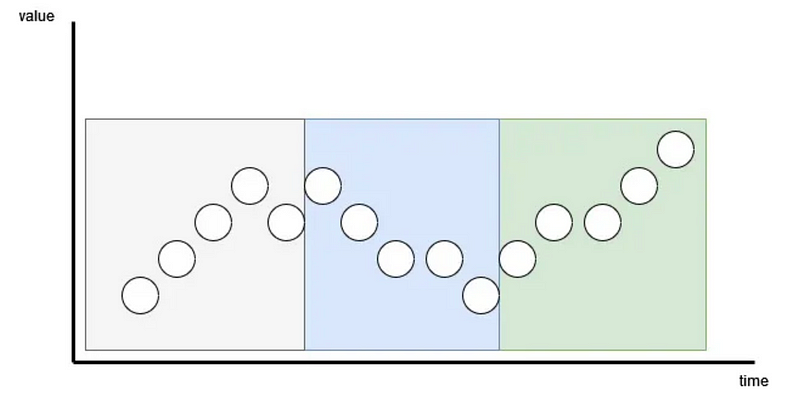
In the figure above, we can see that with patching, we group points of time together and tokenize them. The number of points in patch is determined by the patch length. In the figure above, the patch length is set to five.

This allows the extraction of local semantic meaning. In other words, the model can now learn relationships with past and future time steps. This has also the added benefit of reducing the number of tokens fed to the model, making it faster to train. 

While in PatchTST, the patch length is fixed, in Moirai, the patch length depends on the frequency of the data.

For high-frequency data (every second or minute), the patch length will be larger, to capture more information across time. For low-frequency data (yearly, quarterly), the patch length is smaller. 

The patch length is actually selected by the predefined settings listed below.

Here, Moirai uses a linear layer for the input projection for each patch size. Since there are five possible patch lengths, the model uses up to five different projection layers. 

This means that if pass series with different frequencies, but overlapping patch lengths, this projection layer is shared across series. For example, if we pass a daily and a monthly series, then projection layers for patch lengths 16 and 32 are shared for both series.

Once patched, the series are sent to the encoder-only Transformer and its attention mechanism.

Any-variate attention

To make the model flexible, it is important for the attention mechanism to be able to treat arbitrary multivariate time series.

Learning interdependency in multivariate series is a challenged for Transformer-based models, which often opt for channel independence. This means that each series is treated separately and their influence on each other is not considered.

To overcome this challenge, Moirai simply flattens multivariate series into a long, unique series. That way, all variates are considered in a single sequence.

Of course, this means that the model must be able to distinguish the different series in this long sequence.

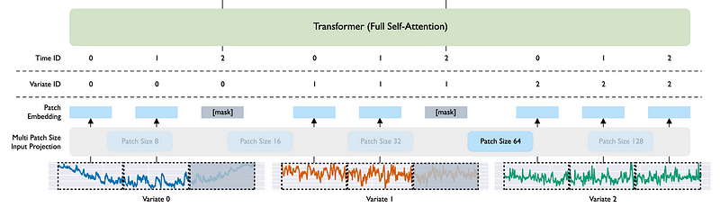
In the figure above, we focus on the input steps of Moirai and notice the Variate ID and Time ID rows. This is how the model can keep track of which values pertain to which series.

The final step is then to generate predictions using a mixture of distributions.

Mixture distribution

A mixture distribution is simply the combination of many distribution functions. It is usually a convex combination, meaning that it is a weighted sum of different distributions, where the sum of the weights equals one, as shown below.

In the equation above, P(x) represents a distribution function and w is the weight assigned to that distribution.

For example, we can visualize what a mixture distribution made of a Student’s T and log-normal distribution would look like given equal weights.

In the figure above, we can see that the mixture distribution is more complex and flexible than if we chose only one.

Therefore, Moirai implements the same concept but using four different distribution functions:

1. Student’s T distribution: shown to be a robust option for many time series,
2. Negative binomial distribution: for positive count data,
3. Log-normal distribution: for right-skewed data, which is common in economics and natural phenomena,
4. Low variance normal distribution: for high confidence predictions.

With this mixture distribution, Moirai tries to create a flexible distribution that can generate reasonable prediction intervals for a wide variety of time series from different domains.

Now that we have a deep understanding of how Moirai works, let’s take a look at the LOTSA dataset and how it was pretrained.

Pretraining Moirai

When working with foundation forecasting models, it is crucial to know the pretraining protocol, as it is a key indicator of the performance of the model. Ultimately, the best models are trained on massive amounts of varied data.

Now, when it comes to building large time models, access to large amounts of data is a big hurdle, as there is simply less time series data than natural language data. 

To overcome this challenge, the researchers have combined 105 open-source time series datasets into a single archive: LOTSA. 

LOTSA stands for Large-scale Open Time Series Archive. This represents one of the largest source of open-source time series data, with more than 27 billion data points.

It contains data from nine different domains like energy, transportation, climate, sales, economics and more.

Moirai was also trained on data at all frequencies, from the second-level, to the yearly frequency. 

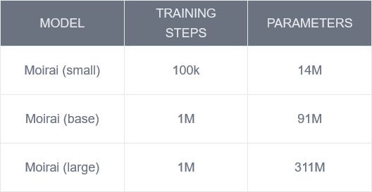
Now, the pretrained Moirai models comes in three different sizes: small, base and large, and their characteristics are summarized in the table below.

It will be interesting to see Moirai in action, as it was trained on probably the largest and most varied open-source time series dataset.

As such, let’s move on and run our own experiment to evaluate the performance of Moirai against other data-specific deep learning models.

Forecasting with Moirai

In this section, we use Moirai in a small forecasting experiment and compare its performance to data-specific deep learning models, like NHITS, NBEATS and TSMixer.

Here, we use a dataset tracking the daily traffic to a blog website. This data was compiled by me, and it is publicly available on GitHub.

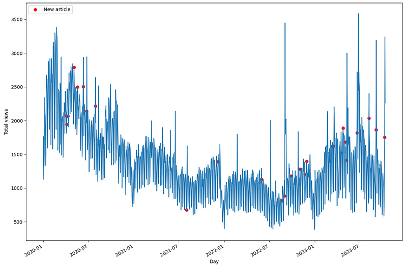
In the figure above, we can see what the data looks like across time. Each red dot represents the date where a new article was published. The dataset also contains information on holidays. 

Thus, it is an interesting scenario to test, as there is a weekly seasonality (more people visit the blog during the week than on the weekend), and we also have the effect of exogenous features, like the publishing of an article and holidays.

As always, the code for this experiment is entirely reproducible and available on GitHub.

Let’s get started!

Initial setup

The first step is of course to import all the necessary packages for this experiment.

Moirai, just like Chronos, can be conviniently installed as a Python package using:

pip install git+https://github.com/SalesforceAIResearch/uni2ts.git

Also, just like Chronos, it relies on methods from GluonTS.

For the deep learning models, we use the neuralforecastpackage, as it offers a simple and intuitive interface to train state-of-the-art models rapidly.

import torch
import numpy as np
import pandas as pd
import matplotlib.pyplot as plt

from gluonts.dataset.multivariate_grouper import MultivariateGrouper
from gluonts.dataset.pandas import PandasDataset
from gluonts.dataset.split import split

from uni2ts.eval_util.plot import plot_single, plot_next_multi
from uni2ts.model.moirai import MoiraiForecast, MoiraiModule

from neuralforecast.core import NeuralForecast
from neuralforecast.models import NHITS, NBEATSx, TSMixerx

from neuralforecast.losses.numpy import mae, mse

import warnings
warnings.filterwarnings('ignore')

Once this is done, we can read the data.

df = pd.read_csv('data/medium_views_published_holidays.csv')
df['ds'] = pd.to_datetime(df['ds'])

Here, the unique_id column is a simple identifier for the series. In this case, we only have one series, so the value is constant.

The ds column holds the date. The y column contains the values of the series, which is the number of visits on the website.

The published column is a flag indicating if a new article was published (1) or not (0). Finally, the is_holiday is another flag indicating if that day is a holiday (1) or not (0).

We are now ready to use perform zero-shot forecasting with Moirai.

Zero-shot forecasting with Moirai

Moirai expects a PandasDataset from GluonTS. Therefore, we must first set the index as the date, and create the PandasDataset.

moirai_df = df.set_index('ds')

ds = PandasDataset.from_long_dataframe(
    moirai_df,
    target='y',
    item_id='unique_id',
    feat_dynamic_real=["published", "is_holiday"]
)

Notice that in the code block above, we specify the feat_dynamic_real parameter with the name of the columns that hold exogenous features. 

Note that these features are available at the time of predicting the future, since we can know when the author will publish, and when the next holiday is.

Once this is done, we split the data into a training and test set. Here, we reserve the last 168 steps for the test set, which gives us 24 windows with a 7-day horizon.

test_size = 168
horizon = 7

train, test_template = split(
    ds, offset=-test_size
)

test_data = test_template.generate_instances(
    prediction_length=horizon,
    windows=test_size//horizon,
    distance=horizon
)

Then, we initialize the Moirai model and make predictions. Due to my limited access to computing power, I am using the small model, but feel free to use the base or large model.

model = MoiraiForecast(
    module=MoiraiModule.from_pretrained(f"Salesforce/moirai-1.0-R-small"),
    prediction_length=horizon,
    context_length=500,
    patch_size="auto",
    num_samples=100,
    target_dim=1,
    feat_dynamic_real_dim=ds.num_feat_dynamic_real,
    past_feat_dynamic_real_dim=ds.num_past_feat_dynamic_real,
)

predictor = model.create_predictor(batch_size=32)
forecasts = predictor.predict(test_data.input)
forecasts = list(forecasts)

In the code block above, notice that we specify the number of samples with the num_samples parameter. Since Moirai is a probabilistic model, it needs to draw many samples to generate a reasonable prediction interval.

Also, the feat_dynamic_real_dim is equal to two, as it corresponds to the number of columns that represents past and future exogenous features. However, the past_feat_dynamic_real_dim is 0, because we do not have exogenous features with information only available in the past.

At this point, the forecast variable is a list of lists. Here, it holds a list for each prediction window, so it has 24 lists.

Inside each list, we have an array containing 100 samples for each forecasting step.

Thus, let’s write a small function to help us format the predictions as a DataFrame and extract a user-defined confidence interval.

def get_median_and_ci(data, 
                      horizon,
                      id,
                      confidence=0.80):

    n_samples, n_timesteps = data.shape
    
    # Calculate the median for each timestep
    medians = np.median(data, axis=0)
    
    # Calculate the lower and upper percentile for the given confidence interval
    lower_percentile = (1 - confidence) / 2 * 100
    upper_percentile = (1 + confidence) / 2 * 100
    
    # Calculate the lower and upper bounds for each timestep
    lower_bounds = np.percentile(data, lower_percentile, axis=0)
    upper_bounds = np.percentile(data, upper_percentile, axis=0)

    # Create a DataFrame with the results
    df = pd.DataFrame({
        'unique_id': id,
        'Moirai': medians,
        f'Moirai-lo-{int(confidence*100)}': lower_bounds,
        f'Moirai-hi-{int(confidence*100)}': upper_bounds
    })
    
    return df

Now, let’s run the function and use an 80% confidence interval.

moirai_preds = [
    get_median_and_ci(
        data=forecasts[i].samples,
        horizon=horizon,
        id=1
    )
    for i in range(24)
]

moirai_preds_df = pd.concat(moirai_preds, axis=0, ignore_index=True)

In the figure above, we can see that we now have predictions nicely formatted as a DataFrame. Note that they were generated through cross-validation, using 24 windows with a horizon of 7.

We can then plot the predictions against the actual values, as shown below.

Here, we notice that Moirai has a lot of trouble forecasting the peaks. In fact, the 80% confidence interval does not even include them. However, those peaks can be seen as anomalies, which makes sense that the model has trouble anticipating them.

Now, let’s use dedicated deep learning models and compare their performance to Moirai.

Full-shot forecasting with deep learning

Here, we use the exact same conditions as with Moirai, but use deep learning models instead.

Specifically, we use NHITS, NBEATS and TSMixer, and we use their implementation available in neuralforecast.

So, let’s initialize each model. Here, we train for a maximum of 1000 steps, but set an early stop patience to three validation checks.

models = [NHITS(h=horizon,
                input_size=5*horizon,
                futr_exog_list=["published", "is_holiday"],
                max_steps=1000,
                early_stop_patience_steps=3,),
         NBEATSx(h=horizon,
                input_size=5*horizon,
                futr_exog_list=["published", "is_holiday"], 
                max_steps=1000,
                early_stop_patience_steps=3,),
         TSMixerx(h=horizon,
                  input_size=5*horizon,
                  n_series=1,
                  futr_exog_list=["published", "is_holiday"],
                  max_steps=1000,
                  early_stop_patience_steps=3)]

Notice above that we use the futr_exog_listwhich contains the name of features available both in the past and in the future at prediction time, just like the feat_dynamic_real parameter with Moirai.

Then, we initialize the NeuralForecastobject and we can launch the cross-validation process, which replicates the setup of Moirai.

nf = NeuralForecast(models=models, freq='D')

preds_df = nf.cross_validation(
    df=df,
    step_size=horizon,
    val_size=168,
    test_size=168,
    n_windows=None
)

Once this is done, we can combine both DataFrames that hold predictions from each models into a single one.

all_preds = preds_df[['NHITS', 'NBEATSx', 'TSMixerx', 'y']]
all_preds['Moirai'] = moirai_preds_df['Moirai'].values

all_preds = all_preds.reset_index(drop=False)

This makes it easy for us to evaluate the performance of each model.

Evaluation

Now, we calculate the mean absolute error (MAE) and symmetric mean absolute percentage error (sMAPE) for each model, using the utilsforecast library.

from utilsforecast.losses import mae, smape
from utilsforecast.evaluation import evaluate

evaluation = evaluate(
    all_preds,
    metrics=[mae, smape],
    target_col='y',
    id_col='unique_id'
)

We can optionally plot each metric for easy comparison.

From the figure above, we can see that Moirai has the worst performance, while TSMixer is the champion model, as it achieves the lowest MAE and sMAPE.

While Moirai shows an underwhelming performance in this scenario, keep in mind that we only tested a single dataset, so it is not a representative evaluation of its performance.

Also, we used the small model, which is the least performance model. Using the base or the large model is likely going to give better results, although the time of inference will likely be longer as well.

Conclusion

Moirai is an open-source foundation forecasting model developed by Salesforce that can perform zero-shot forecasting a wide variety of time series data.

It can be installed as a Python package, and unlike Lag-Llama or Chronos, it supports exogenous features.

The release of Moirai also comes with the LOTSA dataset, which is the largest open-source repository of time series data. This is an important contribution that will greatly speed the developement of large time models, much like what we have witnessed with large language models.

While our experiment resulted in underwhelming performance, keep in mind that using the base or large model will result in better forecasts. 

Still, I believe that each problem requires its own unique solution. As such, make sure to test foundation models and data-specific models, to assess the performance and costs of using each approach.

Thanks for reading! I hope that you enjoyed it and that you learned something new!

Cheers 🍻

Learn the latest time series analysis techniques with my free time series cheat sheet in Python! Get the implementation of statistical and deep learning techniques, all in Python and TensorFlow!

Support me

Enjoying my work? Show your support with Buy me a coffee, a simple way for you to encourage me, and I get to enjoy a cup of coffee! If you feel like it, just click the button below 👇

References

[1] G. Woo, C. Liu, A. Kumar, C. Xiong, S. Savarese, and D. Sahoo, “Unified Training of Universal Time Series Forecasting Transformers.” Accessed: Aug. 13, 2024. [Online]. Available: https://arxiv.org/pdf/2402.02592

Official repository of Moirai — GitHub