Mixture of KAN Experts for High-Performance Time Series Forecasting

The introduction of the Kolmogorov-Arnold Network (KAN) marked an important contribution to the field of deep learning, as it represented an alternative to the multilayer perceptron (MLP). 

The MLP is of course the building block of many deep learning models, including state-of-the-art forecasting methods like N-BEATS, NHiTS and TSMixer.

However, in a forecasting benchmark using KAN, MLP, NHiTS and NBEATS, we discovered that KAN was generally very slow and consistently performed worse on various forecasting tasks. Note that the benchmark was done on the M3 and M4 datasets, which contain more than 99 000 unique time series with frequencies ranging from hourly to yearly. 

Ultimately, at that time, applying KANs for time series forecasting was disappointing and not a recommended approach.

This has changed now with Reversible Mixture of KAN (RMoK) as introduced in the paper: KAN4TSF: Are KAN and KAN-based Models Effective for Time Series Forecasting?

In this article, we first explore the architecture and inner workings of the Reversible Mixture of KAN model and then use it in a small experiment using Python.

As always, for more details, make to read to original paper.

Let’s get started!

Revisiting KAN

Before exploring the architecture of RMoK, let’s first refresh our memory on the inner workings of KAN.

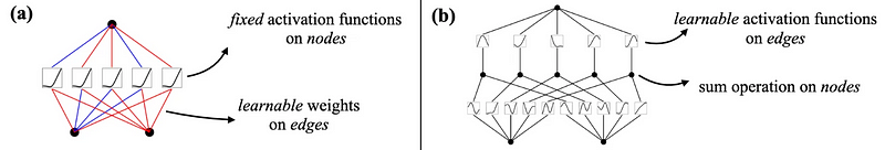
In the figure above, we see a direct comparison between the MLP and the KAN. In the MLP, the edges represent learnable weights, and the nodes are fixed activation functions, like ReLU, tanh, etc.

On the other hand, the KAN uses learnable activation functions on the edges and the nodes are summation operations of those functions.

This is the Kolmogorov-Arnold representation theorem in effect, as it states that multivariate functions can be represented by the combination of univariate functions. 

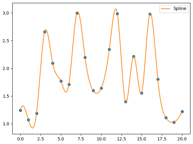
Specifically, KAN uses B-splines as learnable function to model non-linear data. This gives flexibility to the model and allows it to learn complex non-linear relationships, as shown in the figure below.

While splines are flexible functions, researchers have proposed many variants to further expand the applications of KAN and its performance. 

Among those variants are the Wav-KAN, JacobiKAN and TaylorKAN, which are all used in the RMoK model.

Wav-KAN

The Wav-KAN uses wavelet functions instead of splines. These are particularly useful in treating signals, like time series, as they can extract both frequency and location information.

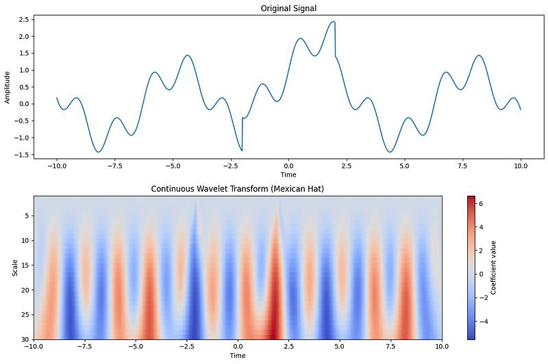
In the figure above, we can see how the Ricker wavelet (also known as the Mexican Hat wavelet) transforms the input signal shown in the top plot to the bottom plot. 

Notice that the bottom plot exhibits oscillatory changes, just like in the signal. Also, around the -2.5 and 2.5 mark, the colors are particularly dark. These indicate sudden changes in the signal in the top plot.

Thus, we can see how the Wav-KAN is particularly suited for time series data, as it detects positional and frequency changes.

JacobiKAN and TaylorKAN

Splines are not the only functions that can be used to approximate other functions. 

Jacobi polynomials and Taylor polynomials are also popular approaches for function approximation, resulting in the JacobiKAN and TaylorKAN.

TaylorKAN

Without diving deep into mathematical complexities, a Taylor polynomial is, by definition, an approximation of a function represented by an infinite sum of its derivatives at an expansion point. The expansion point is where the derivative of both the function and the approximation will be equal.

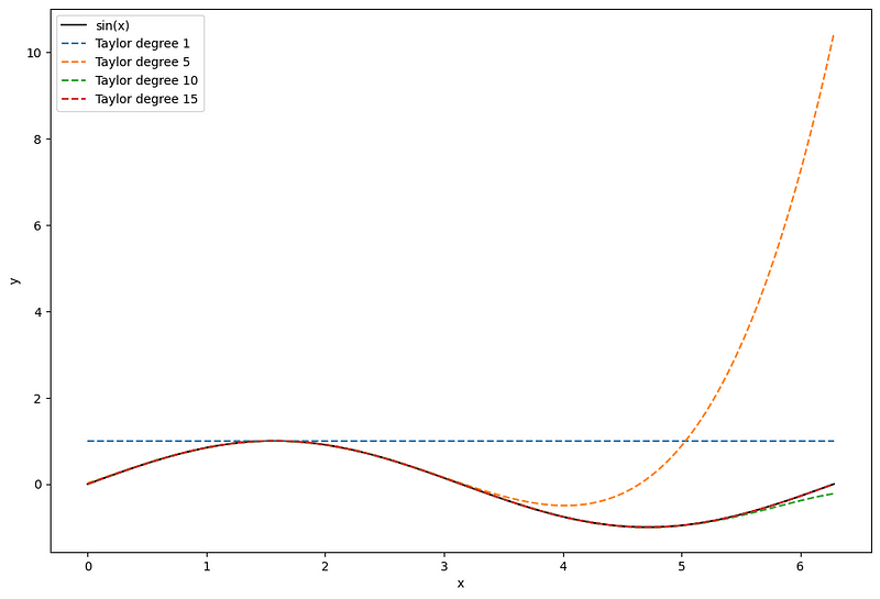
In the figure above, we illustrate the approximation of the sin(x) function using Taylor polynomials, where 𝜋/2 is the expansion point. Notice how the derivative of all approximations and sin(x) are equal at 𝜋/2. 

Of course, as the degree increases, meaning that more terms are added in the infinite sum, the approximation gets better. However, notice how the approximation quickly degrades as we move further away from the expansion point.

JacobiKAN

Then, Jacobi polynomials form a basis which we can combine and use to approximate more complex functions, a bit like B-splines.

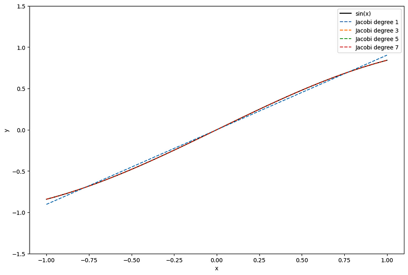
In the figure above, we again approximate sin(x), this time using Jacobi polynomials. Once more, we notice that higher degree polynomials result in better approximations.

Now, notice how the Jacobi polynomials provide a more balanced approximation across the entire function compared to using Taylor approximations.

As such, Jacobi polynomials are better for global approximations, and their errors are often evenly distributed. On the other hand, Taylor polynomials are better for local approximations.

Thus, we can see how combining Wav-KAN for signal processing, JacobiKAN for accurate global approximations, and TaylorKAN for local approximations, can potentially result in learning complex relationships in time series data.

This is exactly the idea that is applied in the Reversible Mixture of KAN model.

Exploring the Reversible Mixture of KAN (RMoK) model

The Reversible Mixture of KAN is a simple model that combines a gating network with a single “mixture of KAN” layer made of different expert KAN layers. Its complete architecture is shown below.

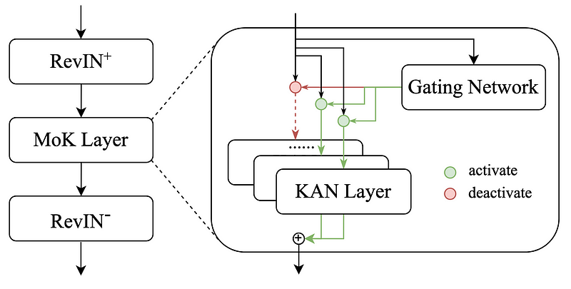
In the figure above, we notice that the model uses RevIN which stands for Reversible Instance Normalization. This is a popular preprocessing technique to handle non-stationary time series data that greatly improves the performance of forecasting models.

So, the data, which flows from top to bottom in the figure above, is first normalized using RevIN, and it enters the Mixture of KAN (MoK) layer.

The MoK layer is composed of a gating network and different layers of Wav-KAN, JacobiKAN and TaylorKAN. 

The gating network is responsible for activating the right layers for specific parts of the data. Then, each expert can learn different temporal features from the data:

• Wav-KAN learns frequency and positional features
• JacobiKAN learns long-term changes
• TaylorKAN learns local short-term changes

Then, the predictions from each expert is combined to form a forecast.

Note that this was done on normalized data. The output of the MoK layer is then denormalized, and we thus obtain the final forecast of the model.

We see that the overall idea and logic behind RMoK is fairly simple. The main difficulty is in selecting the right “experts” for time series forecasting, and the three experts mentioned above seem to be great candidates for the task.

Now that we have a deep understanding of RMoK, let’s apply it in our own experiment using Python.

Forecasting with RMoK

For this section, we apply the RMoK model for long-horizon forecasting and compare its performance to PatchTST, iTransformer and TSMixer.

For this experiment, we use the Electricity Transformer dataset (ETT) released under the Creative Commons License. This tracks the oil temperature of an electricity transformer from two regions in a province of China. For both regions, we have a dataset sampled at each hour and every 15 minutes, for a total of four datasets. In our case, we only use the two datasets sampled at every 15 minutes (ETTm1 and ETTm2).

Here, I extended the neuralforecast library with an adapted implementation of the RMoK model from their official repository. That way, we have a streamlined experience for using and testing different forecasting models.

Note that at the time of writing this article, RMoK is not in a stable release of neuralforecast just yet.

To reproduce the results, you may need to clone the repository and work in this branch.

If the branch is merged, then you can run:

pip install git+https://github.com/Nixtla/neuralforecast.git

As always, the code for this experiment is available on GitHub.

Let’s get started!

Initial setup

The natural first step is to import the required packages. Here, we use neuralforecast to train and predict with each model, and we use utilsforecast to evaluate the models. 

import pandas as pd
import numpy as np
import matplotlib.pyplot as plt

from datasetsforecast.long_horizon import LongHorizon

from neuralforecast.core import NeuralForecast
from neuralforecast.losses.pytorch import MAE, MSE
from neuralforecast.models import TSMixer, PatchTST, iTransformer, RMoK

from utilsforecast.losses import mae, mse
from utilsforecast.evaluation import evaluate

Then, let’s create a helper function that reads the datasets and returns the correct frequency, and test and validation splits. These splits are what is used in the academic literature.

def load_data(name):
    if name == 'Ettm1':
        Y_df, *_ = LongHorizon.load(directory='./', group='ETTm1')
        Y_df['ds'] = pd.to_datetime(Y_df['ds'])
        freq = '15T'
        h = 96
        val_size = 11520
        test_size = 11520
    elif name == 'Ettm2':
        Y_df, *_ = LongHorizon.load(directory='./', group='ETTm2')
        Y_df['ds'] = pd.to_datetime(Y_df['ds'])
        freq = '15T'
        h = 96
        val_size = 11520
        test_size = 11520

    return Y_df, h, val_size, test_size, freq

Note that we use a forecast horizon of 96 time steps for this project.

Great! At this point, we have everything ready to start our experiment.

Training and forecasting with all models

Now, let’s start a for loop to forecast on both datasets.

DATASETS = ['Ettm1', 'Ettm2']

for dataset in DATASETS:

    Y_df, horizon, val_size, test_size, freq = load_data(dataset)

Then, we initialize each model. Here, we use the same configuration as in their respective papers to ensure optimal performances for each model. Thus, we initialize RMoK as:

DATASETS = ['Ettm1', 'Ettm2']

for dataset in DATASETS:

    Y_df, horizon, val_size, test_size, freq = load_data(dataset)

    rmok_model = RMoK(input_size=horizon,
                      h=horizon, 
                      n_series=7,
                      num_experts=4,
                      dropout=0.1,
                      revine_affine=True,
                      learning_rate=0.001,
                      scaler_type='identity',
                      max_steps=1000,
                      early_stop_patience_steps=5)

Notice that we use four experts here, which are Wav-KAN, JacobiKAN, TaylorKAN and a simple MLP. The learning rate is set to 0.001 as per the original paper. 

Also, we allow the model to train for 1000 steps, and set early stopping to five checks. Thus, if the validation loss does not improve five times in a row, the model stops training.

Then, we initialize the rest of the models using their optimal configurations from their respective papers.

DATASETS = ['Ettm1', 'Ettm2']

for dataset in DATASETS:

    Y_df, horizon, val_size, test_size, freq = load_data(dataset)

    rmok_model = RMoK(input_size=horizon,
                      h=horizon, 
                      n_series=7,
                      num_experts=4,
                      dropout=0.1,
                      revine_affine=True,
                      learning_rate=0.001,
                      scaler_type='identity',
                      max_steps=1000,
                      early_stop_patience_steps=5)
    
    patchtst_model = PatchTST(input_size=horizon, 
                              h=horizon, 
                              encoder_layers=3,
                              n_heads=4,
                              hidden_size=16,
                              dropout=0.3,
                              patch_len=16,
                              stride=8,
                              scaler_type='identity', 
                              max_steps=1000, 
                              early_stop_patience_steps=5)
    
    iTransformer_model = iTransformer(input_size=horizon, 
                                      h=horizon, 
                                      n_series=7,
                                      e_layers=2,
                                      hidden_size=128,
                                      d_ff=128,
                                      scaler_type='identity', 
                                      max_steps=1000, 
                                      early_stop_patience_steps=3)
    
    tsmixer_model = TSMixer(input_size=horizon,
                            h=horizon,
                            n_series=7,
                            n_block=2,
                            dropout=0.9,
                            ff_dim=64,
                            learning_rate=0.001,
                            scaler_type='identity',
                            max_steps=1000,
                            early_stop_patience_steps=5)

Then, we can initialize the Neuralforecast object that will handle the training and forecasting procedures for us. Note that we do this within the same for loop.

    models = [rmok_model, patchtst_model, iTransformer_model, tsmixer_model]

    nf = NeuralForecast(models=models, freq=freq)

After, we use cross-validation to generate predictions across different windows in the for loop.

    nf_preds = nf.cross_validation(df=Y_df, val_size=val_size, test_size=test_size, n_windows=None)
    nf_preds = nf_preds.reset_index()

Finally, we save the predictions to CSV files, again in the same for loop.

    evaluation = evaluate(df=nf_preds, metrics=[mae, mse], models=['RMoK', 'PatchTST', 'iTransformer', 'TSMixer'])
    evaluation.to_csv(f'{dataset}_results.csv', index=False, header=True)

Once all of this code runs, we obtain the performance for each model on each series in the dataset.

Evaluation

At this point, each model was trained and used to make predictions. We can then evaluate their performance on both datasets. 

Here, we calculate the mean absolute error (MAE) and mean squared error (MSE).

ettm1_eval = pd.read_csv('Ettm1_results.csv')
ettm1_eval = ettm1_eval.drop(['unique_id'], axis=1).groupby('metric').mean().reset_index()

ettm2_eval = pd.read_csv('Ettm2_results.csv')
ettm2_eval = ettm2_eval.drop(['unique_id'], axis=1).groupby('metric').mean().reset_index()

We can then optionally plot the metrics in bar plots, or report them in a table as shown below.

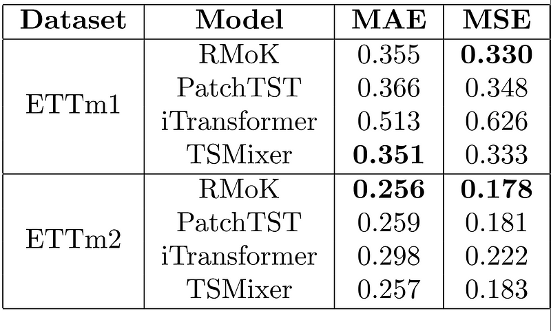
In the table above, we report the MAE and MSE for each model on each dataset. The lower the value, the better the performance, and the best values are shown in bold.

Here, we see that for a horizon of 96 time steps, the RMoK model achieves the best MSE in ETTm1, and it is the champion model for ETTm2. 

Thus, from this experiment, we see that RMoK can definitely rival some of the best forecasting methods like TSMixer and PatchTST, which is a much more positive outcome than our first experiment with the simple KAN model.

Clearly, using different learnable activation functions in dedicated KAN layers and combining them boosts the performance of KAN-based models in time series forecasting tasks.

Conclusion

In this article, we discovered the Reversible Mixture of KAN (RMoK), a fundamentally simple model that combines different KAN layers that specialize in specific parts of the data to perform time series forecasting.

Specifically, the model uses Wav-KAN, which uses wavelet functions to extract frequency and positional information. It also uses JacobiKAN and TaylorKAN, which are good for global and local approximations respectively, allowing the model to capture long-term changes and local short-term changes.

Combining these layers as a mixture of experts yields a model that can performs very well on forecasting tasks.

Keep in mind that our experiment is meant to show how to use RMoK with Python, and it does not represent a comprehensive benchmark. However, the results are encouraging and I believe that RMoK is a model worth trying on your projects.

As always, each problem requires its own solution, and now you can test if RMoK is the best answer to your scenario.

Thanks for reading! I hope that you enjoyed it and that you learned something new!

Learn the latest time series analysis techniques with my free time series cheat sheet in Python! Get the implementation of statistical and deep learning techniques, all in Python and TensorFlow!

Cheers 🍻

Support me

Enjoying my work? Show your support with Buy me a coffee, a simple way for you to encourage me, and I get to enjoy a cup of coffee! If you feel like it, just click the button below 👇

References

[1] X. Han, X. Zhang, Y. Wu, Z. Zhang, and Z. Wu, “KAN4TSF: Are KAN and KAN-based models Effective for Time Series Forecasting?” Accessed: Sep. 09, 2024. [Online]. Available: https://arxiv.org/pdf/2408.11306

[2] Z. Liu et al., “KAN: Kolmogorov-Arnold Networks.” Available: https://arxiv.org/pdf/2404.19756

[3] Official implementation of RMoK — GitHub